Deep Learning-Based Anomaly Detection Using PyTorch

Anomaly detection refers to the problem of finding patterns that do not conform to expected behavior. These non-conforming patterns are known as anomalies, outliers, discordant observations, exceptions, aberrations, surprises, or contaminants in different application domains.

Anomaly detection is used across many industries to identify critical events or observations that can significantly deviate from the norm. It has widespread applications in credit card fraud detection, health insurance claims analysis, damage or defects detection in manufacturing, network intrusion detection, and other domains where identifying anomalies provides immense business value.

For example, anomaly detection plays a vital role in healthcare. Analyzing patient data can help flag anomalous records that may indicate medical conditions or diseases. Detecting network intrusions or cyber attacks against a system early is crucial to prevent security breaches. In ecommerce, accurately finding anomalies in customer transactions can detect fraudulent purchases and prevent financial losses.

The goal of anomaly detection is to build models that can accurately distinguish between normal and anomalous data points. Anomalies are rare events compared to normal data instances. This class imbalance makes anomaly detection a challenging machine learning problem.

Over the past decade, deep learning techniques have emerged as a preferred approach for anomaly detection across different applications. Deep neural networks have the ability to learn complex representations and patterns within high-dimensional data like images, text, time series, and more. This makes deep learning well-suited for tackling the intricacies of identifying anomalies.

In this article, we will focus on building a PyTorch anomaly detector based on deep learning. We will learn about the various techniques and architectures used for anomaly detection. Then we will implement and train an autoencoder model on an open dataset using PyTorch to identify anomalies.

Anomaly Detection Methods

Anomaly detection has been an important problem in various domains such as fraud detection, system health monitoring, and network intrusion detection. There are two main approaches for detecting anomalies:

Traditional Statistical Methods

Traditional statistical methods for anomaly detection make assumptions about the distribution of the data. Common statistical techniques include measuring outliers based on statistical metrics like mean and standard deviation, as well as density-based techniques. These methods work well when the assumptions hold, but do not generalize well when the data distribution changes over time. They also tend to perform poorly with high-dimensional data.

Machine Learning Based Methods

More recent techniques use machine learning models to learn the patterns of normal data during training. During inference, these models can detect significant deviations from normal patterns as anomalies. Common machine learning techniques include clustering algorithms like k-means, as well as neural network models like autoencoders. A key advantage of machine learning methods is the ability to learn complex patterns in high-dimensional data without requiring explicit assumptions about data distribution. However, these methods require sufficiently large and representative training data.

In summary, traditional statistical methods rely on assumptions about data distribution, while machine learning methods learn patterns from data directly. Machine learning techniques have become more popular for anomaly detection, especially with the availability of larger datasets.

Deep Learning for Anomaly Detection

Deep learning methods like autoencoders, GANs, and other neural network architectures have become popular techniques for anomaly detection in recent years. There are several key advantages that make deep learning well-suited for identifying anomalies:

Feature learning: Deep learning models can automatically learn complex features and patterns from raw data that are useful for detecting anomalies. This removes the need for manual feature engineering.
Nonlinear modeling: Neural networks can model complex nonlinear relationships in data. Many real-world anomaly detection tasks involve highly nonlinear and complex data.
Scalability: Deep learning models can be applied to large and high-dimensional datasets common in anomaly detection. The distributed training capabilities make them highly scalable.
Unsupervised learning: Many deep anomaly detection models are unsupervised, so they can be trained without normal/anomaly labeled data. This is important since labeled data is often scarce in anomaly detection.
Representational power: Deep neural networks have proven capable of learning powerful representations of highly complex data like images, video, audio and text. This makes them suitable for anomaly detection across diverse problem domains.
Transfer learning: Pretrained neural networks can be fine-tuned to perform anomaly detection in a specific application domain, avoiding training large models from scratch.

Some popular deep learning techniques used for anomaly detection include autoencoders, Generative Adversarial Networks (GANs), Deep Belief Networks (DBNs), recurrent neural networks (RNNs) and Long Short Term Memory Networks (LSTMs). Overall, deep learning has opened up powerful new approaches for identifying unusual data instances, patterns, and behaviors across many real-world applications.

Introduction to PyTorch

PyTorch is an open source machine learning framework based on Python that enables fast, flexible experimentation. It provides a relatively simple way to build neural networks using an imperative, define-by-run approach that feels more like Python.

Some of the key features of PyTorch include:

Tensors --- The main data structure in PyTorch is the tensor. Tensors are similar to NumPy arrays and support advanced GPU acceleration capabilities. They also support automatic differentiation using autograd.
Autograd --- This is PyTorch's automatic differentiation engine that allows you to dynamically compute gradients. It is extremely useful for building and training neural networks.
Neural network modules --- PyTorch provides neural network layers through the nn module. These are modular and composable to allow you to build custom architectures easily. Some common modules include convolutional layers, RNNs, linear layers etc.
Optimizers --- Optimization algorithms like SGD, Adam, RMSProp etc. come built-in with PyTorch. This makes the training process easy and efficient.
Built for GPUs --- PyTorch is built to utilize GPUs seamlessly with features like CUDA tensors. Using GPUs can provide significant speedups during model training.

Overall, PyTorch provides a flexible framework that feels more native to Python and enables fast prototyping and experimentation. The combination of tensor computations, autograd and nn makes it very well suited for deep learning research and applications.

Implementing Autoencoder in PyTorch

Autoencoders are a type of neural network architecture that are often used for anomaly detection. The goal of an autoencoder is to learn to reconstruct its inputs, which forces it to learn useful properties about the data.

Autoencoders consist of two main components --- an encoder and a decoder. The encoder compresses the input into a lower-dimensional code. The decoder then reconstructs the input from this compressed code. By training the autoencoder to minimize the difference between the input and reconstructed input, the autoencoder learns to effectively encode the most useful properties of the data.

To implement an autoencoder in PyTorch, we first define the encoder and decoder networks. The encoder typically consists of linear layers followed by activation functions like ReLU to introduce non-linearities. The decoder mirrors the encoder by reversing the order of the linear layers and activations.

For the loss function, we want to compare the reconstructed input to the original input. A common choice is mean squared error (MSE) loss, which computes the pixel-wise error between the reconstructed image and original image. We initialize the model parameters randomly, then train the autoencoder by looping through batches of data, doing a forward pass to generate reconstructions, computing the loss, and updating the model parameters with backpropagation.

By training the autoencoder to minimize the MSE between input and reconstruction, it will learn to efficiently compress the input into the code layer in a way that preserves the most useful information to recreate the original input. This allows the autoencoder to learn useful properties and patterns in the training data.

Training the Autoencoder

To train the autoencoder, we first need to prepare the training data. This involves loading the dataset and transforming it into a PyTorch tensor. We can use common datasets like MNIST or CIFAR10 for anomaly detection.

Next, we define the training loop. This will iterate through the dataset in batches and train the model. We first do a forward pass of the input batch through the encoder and decoder parts of the model. Then we calculate the reconstruction loss, which measures how well the decoder was able to reconstruct the input from the encoded representation. Common loss functions are MSELoss or BCELoss.

The next key part is optimization. We use an optimizer like Adam or SGD to update the model weights and minimize the reconstruction loss. This is done by computing the gradients of the loss with respect to the weights, and then updating the weights accordingly. The learning rate determines how big of an update is made at each iteration.

Some other important training loop components are:

Tracking metrics like loss over iterations to monitor training progress
Saving model checkpoints periodically to allow resuming training if needed
Validation --- evaluate model on hold-out set to track generalization

With the training loop implemented, we can now train the autoencoder model on the prepared data for a number of epochs until the reconstruction loss converges. Once trained, we can evaluate the model's anomaly detection performance. The autoencoder will reconstruct normal data well but have high reconstruction error for anomalous inputs.

Evaluating the Autoencoder

Once the autoencoder is trained, it's crucial to evaluate how well it performs at detecting anomalies. There are several key metrics we can use:

Reconstruction Error

The reconstruction error measures how well the autoencoder can reconstruct normal data. We pass the normal validation samples into the encoder and decoder to get the reconstructed output. Then we compare the reconstructed output to the original input using a loss function like MSE. The lower the reconstruction error, the better the autoencoder has learned to reproduce normal data.

Precision and Recall

Precision measures what percentage of positive identifications were correct. Recall measures what percentage of actual positives were correctly identified. We pass anomalous data into the trained autoencoder and threshold the reconstruction error to identify anomalies. Then we can compare to the true labels to calculate precision and recall. The higher the precision and recall, the better the model is at detecting anomalies.

ROC Curve

The receiver operating characteristic (ROC) curve plots the true positive rate (recall) against the false positive rate as we vary the reconstruction error threshold. The area under the ROC curve quantifies how well the model distinguishes between normal and anomalous data. An area of 1 represents perfect classification, while an area of 0.5 is equivalent to random guessing. We want the area under the ROC curve to be as close to 1 as possible.

Analyzing these metrics helps evaluate how well the autoencoder model performs at identifying anomalies compared to normal data. We can use this analysis to determine if we need to adjust the model architecture or training process to improve detection performance. The ultimate goal is to optimize reconstruction error, precision, recall and the ROC curve.

Improving the Autoencoder

Autoencoders can be improved in various ways to detect anomalies more accurately. Some techniques include:

Overcomplete autoencoders --- Using more nodes in the hidden layer than input/output layers creates a bottleneck that forces the autoencoder to learn a more robust compression. This can improve reconstruction of normal data while anomalies remain poorly reconstructed.
Denoising autoencoders --- Adding noise to input data trains the autoencoder to reconstruct the original from noisy inputs. This makes it better at learning useful patterns in data rather than memorizing and recapitulating inputs.
Adversarial training --- A discriminator network is trained to differentiate between real samples and those reconstructed by the autoencoder. The autoencoder is then updated to generate reconstructions that can fool the discriminator. This makes the autoencoder outputs closer to the real data distribution.
Variational autoencoders --- VAEs impose constraints on the hidden layer to conform to a chosen prior distribution. This regularization prevents the autoencoder from simply learning to copy inputs, improving generalization.
Robust deep autoencoders --- Adding an extra penalty term based on relative reconstruction error makes the autoencoder focus more on anomalies with large deviations.

Carefully chosen techniques like these can significantly boost the anomaly detection performance of autoencoders. Overcomplete and denoising autoencoders are relatively simple to implement, while adversarial training and VAEs require more sophisticated networks but can provide powerful improvements.

Deploying the Model

Once we have trained our anomaly detection model, the next step is to deploy it so it can be used to analyze new data. There are a few main steps to deploying a PyTorch model:

Exporting the Trained Model

PyTorch models are trained in Python but for deployment we need to export them to a serialized format. This allows the model to be loaded in a production environment. A common format is ONNX (Open Neural Network Exchange). We can export our trained autoencoder model like this:

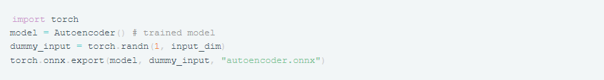
This exports the model architecture and weights into the autoencoder.onnx file.

Writing Prediction Code

Next we need some code to load the ONNX model and run predictions on new data. This will deserialize the model and we can pass it input data like:

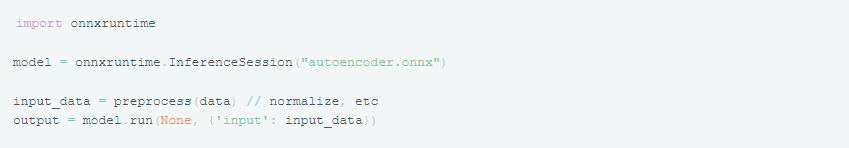
The output will contain anomaly scores for the new data.

Model Serving

For scalable deployment, we need to serve the model via an API. This allows sending requests to get predictions. Options include:

Docker container with REST API
Serverless functions like AWS Lambda
Realtime serving via TensorFlow Serving

The exported ONNX model can be loaded on startup and the prediction code called in the API handler. This enables integrating anomaly detection into applications.

Overall, exporting the model, writing prediction code, and model serving enable putting an anomaly detector into production. This allows continuously monitoring new data flowing into the system.

Conclusion

Anomaly detection is an important capability in many applications such as fraud detection, system health monitoring, and predictive maintenance. Deep learning techniques like autoencoders can learn complex representations of normal data and detect anomalies effectively.

In this article, we implemented an autoencoder anomaly detection model in PyTorch. We trained it on normal data, evaluated it, and improved its performance by tuning hyperparameters. The model can now be deployed to detect anomalies in new data.

While autoencoders work well, there are some limitations. They may not perform as well on complex and high-dimensional data. Novel deep learning architectures can be explored to handle such cases better.

The model can be further improved by using larger and more representative datasets for training. Advanced sampling and weighting techniques may help improve performance on imbalanced data. Other semi-supervised and unsupervised methods can also be evaluated as alternatives.

Overall, deep learning has opened up new possibilities for building highly accurate and robust anomaly detection systems. With the power of PyTorch and other frameworks, these models can be rapidly developed, deployed and scaled. There are ample opportunities for innovation in this exciting field.