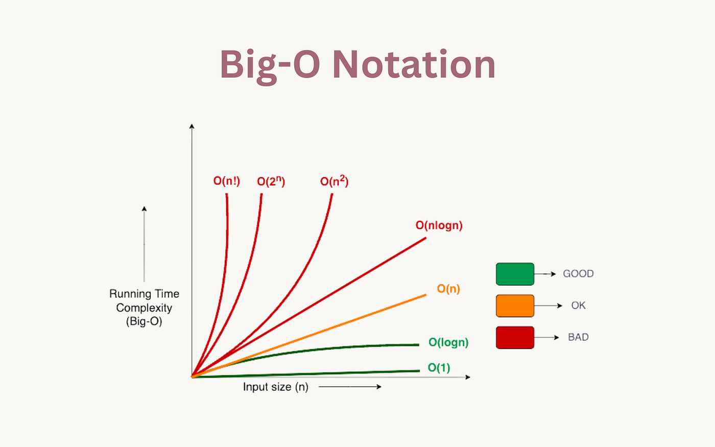
In mathematics, there are often multiple ways to arrive at the answer to a particular problem; similarly, in programming, algorithms can be implemented in various ways, and even though they may accomplish the same purpose, some algorithms perform more efficiently than others. Let’s define some key terminologies so we are all on the same page.
An algorithm is a set of rules or processes that computers follow to solve problems. For instance, you could write an algorithm to find the average in a given list of numbers. Big O notation is simply a mathematical representation used to describe or measure the performance of an algorithm. These are terms you’ll come across often as a software developer. This article aims to give you a good understanding of Big O notation and how to accurately evaluate algorithms to enable you to spot poor algorithms in your programmes and write better ones.
Why The Need for Big O Notation
Many factors influence how long a piece of code takes to run, like the machine you’re using, the programming language, and maybe even the weather, time of day, or your nationality (just kidding about those last three). Big O notation ignores all that and focuses on how the number of operations increases as your input grows, assuming the worst-case scenario.
An algorithm described as O(n) (pronounced “Big O of n”) indicates that the number of operations or steps increases directly with the size of the input — 100 inputs might result in 100 operations, while a million inputs could lead to a million operations. Conversely, O(n²) indicates the complexity grows in proportion to the square of the input size — 10 inputs might lead to 100 operations, and 1,000 inputs could result in a million operations.
Types of Big O Notations
The two Big O notations mentioned above are very common, and most algorithms fall into one of these categories. However, Big O notations can be classified into seven main types, ranked from best to worst:
- O(1) — Constant
- O(log n) — Logarithmic
- O(n) — Linear
- O(n log n) — Quasilinear
- O(n²) — Quadratic
- O(2ⁿ) — Exponential
- O(n!) — Factorial
When evaluating the performance of an algorithm, we typically consider two primary factors: time complexity and space complexity. Time complexity describes how the running time of an algorithm grows as the input size increases, while space complexity describes how much memory the algorithm uses during execution. These measures help compare algorithms to understand how efficiently they solve a problem. Both are defined using the Big O notation types listed above, and usually require a trade-off commonly known as the space-time trade-off. For example, an algorithm might achieve O(1) time complexity at the cost of O(n) space complexity.
Let’s go over each of the categories, explaining what they mean, and common examples of algorithms in that category.
I will be using TypeScript as the programming language in the examples, but the same principle holds for any programming language.
1. O(1) — Constant Time/Space
Algorithms in this category require the same number of steps, amount of space, or execution time regardless of the input size. The key distinction is that *“constant” *refers to a consistent number of operations, not necessarily just one. Whether the process involves ten steps or a thousand, it remains in this category as long as the input size does not determine the total resource consumption.
Consider this example;
function getFirstElement<T>(arr: T[]): T {
  return arr[0];
}
Whether arr has 10 elements or 10 million, accessing arr[0] is a single lookup. The size of arr never enters the calculation, so the work stays flat — hence O(1) for both time and space complexities.
How accessing array elements by index works
Accessing an element in an array by its index is a constant-time operation, O(1), regardless of the element’s position or the total size of the array. This efficiency is due to the way arrays are allocated in contiguous memory blocks. Because the memory is sequential, the computer can calculate the exact memory address of any element using a simple mathematical formula: memory(index)= startingAddress + (index × itemSize)
This direct calculation allows for immediate access without having to traverse the entire array.
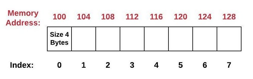
To find the fifth item (index 4) using this formula, computers typically do:
memory(4) = 100 + (4 × 4) = 116
And so, it knows to look at address 116 for the 5th item without searching through the array.
function logHello<T>(arr: T[]): T {
  console.log(arr.length)
  for(let i = 0; i<1000; i++) console.log('Hello')
}
The above example can be quite tricky, especially to some who may think algorithms involving loops are classified as O(n), but this algorithm only follows 1,001 steps — logging the total number of items in the input array and “hello” 1,000 times. Even if the array has a million items, it’ll still take 1,001 steps to run.
Other common constant-time operations include:
- Using Array.push and Array.pop methods to add or remove the last item in an array.
- Accessing object properties.
- Getting or setting items in a Map.
2. O(log n) — Logarithmic Time/Space
Algorithms in this category scale efficiently because they discard a significant portion of the remaining data at each step rather than checking every item. This logarithmic approach ensures that the total number of operations increases by only one each time the input size doubles.
A common example is the Binary Search algorithm that searches a sorted array by repeatedly halving the search space.
function binarySearch(arr: number[], target: number): number {
  let low = 0, high = arr.length - 1;

  while (low <= high) {
    const mid = Math.floor((low + high) / 2);

    if (arr[mid] === target) return mid;
    if (arr[mid] < target) low = mid + 1;
    else high = mid - 1;
  }

  return -1; // Target not found
}
A better way to calculate the middle element (mid) to avoid buffer overflow is:
Math.floor(low + (high — low)/2)
Each time through the loop, the search space is cut in half. If arr has 1,000 elements, after one comparison, you're only considering 500, then 250, then 125, and so on, until you're down to one. This only works because the array is sorted — the algorithm can safely throw away half the elements at each step, knowing the target can't be there.
How the halving actually adds up
If you start with n elements and keep dividing by 2, the number of times you can do that before reaching 1 is log₂(n). For example, 1,000 elements require about 10 comparisons, while 1,000,000 need about 20. Increasing your input size by a thousand adds only around 10 more steps. That’s why binary search on an array with a billion items still wraps up in roughly 30 comparisons.
Other common logarithmic operations:
- Searching, inserting, and deleting elements in balanced binary search trees (BSTs).
- Querying B-trees, the primary data structure used by databases and file systems for efficient indexing and retrieval.
- Fast exponentiation (exponentiation by squaring), which calculates x^n through repeated squaring rather than linear multiplication.
3. O(n) — Linear Time/Space
This is the most common classification, where, as mentioned earlier, the operations in these algorithms increase linearly with the size of the input.
Consider this example for finding the largest number in an array.
function findMax(arr: number[]): number {
  let max = arr[0];

  for (let i = 1; i < arr.length; i++) {
    if (arr[i] > max) max = arr[i];
  }

  return max;
}
The loop executes once for each element after the first. With n elements, that’s n — 1 iterations, and since constants and small offsets are ignored in Big O notations, it simplifies to O(n).
Can you come up with a better algorithm here?
To know the maximum value in a list, you have to look at every value at least once — if you skip even one, it could turn out to be the largest and you’d never know. So O(n) isn’t just what this particular implementation happens to do, it’s the best any algorithm can do for this problem.
Consider this example and determine the Big O notation:
function sumAndProduct(arr: number[]): { sum: number; product: number } {
  let sum = 0;
  for (const num of arr) sum += num;

  let product = 1;
  for (const num of arr) product *= num;

  return { sum, product };
}
It may be tempting to say O(n²), especially if you’re used to spotting nested loops as a red flag. But these loops aren’t nested — they run one after the other, not one inside the other. That’s n + n = 2n total steps, and since Big O ignores constants, 2n simplifies to O(n).
Other common linear operations:
Array.map,Array.filter,Array.reduce,Array.forEach, and most array methods that involve checking conditions across all elements.- Searching for an item in an unsorted array.
- Calculating the sum or average of a list.
**4. O(n log n) — **Quasilinear/Linearithmic Time
This complexity appears mainly in efficient sorting algorithms — it’s the sweet spot between the slow O(n²) sorts and the faster O(n) ones, offering a speed that no comparison-based sort can actually reach.
A classic example of this algorithm is merge sort, where the unsorted array is divided into two halves, each half is sorted recursively, and then the sorted halves are merged back together into one sorted array.
function mergeSort(arr: number[]): number[] {
// Base case: arrays with 0 or 1 element are already sorted
  if (arr.length <= 1) return arr;

  const mid = Math.floor(arr.length / 2);
  const left = mergeSort(arr.slice(0, mid)); // Recursively sort the left half
  const right = mergeSort(arr.slice(mid)); // Recursively sort the right half
  return merge(left, right);
}

// Helper function to merge two sorted arrays into one sorted array
function merge(left: number[], right: number[]): number[] {
  const result: number[] = [];
  let i = 0, j = 0;

// Compare elements from both arrays and push the smaller one
   while (i < left.length && j < right.length) {
    if (left[i] < right[j]) {
      result.push(left[i++]);
    } else {
      result.push(right[j++]);
    }
  }

  // Add any remaining elements from left or right array
  return result.concat(left.slice(i)).concat(right.slice(j));
}
To better understand this algorithm through visualization, checkout this YouTube video: https://youtu.be/V3LGH8T614k?si=M_zQVNXUBPz5TLNY
Where the n and the log n each come from
The array is repeatedly halved until each piece contains a single element. This is similar to the halving pattern from binary search, so it takes log n levels of splitting. But at each of these levels, the merge process iterates through all n elements to reassemble them in order. Performing n work across log n levels results in a total complexity of O(n log n).
It’s easy to look at the recursion and assume it must be O(2ⁿ) (exponential), because each call triggers two more, the key difference is that each call handles only half the data. The total work per level remains constant at n; it is simply distributed across an increasing number of smaller sub-problems.
Other common linearithmic operations:
- Quicksort which can be similar to merge sort on average (its worst case is O(n²), which is a separate conversation; you’re welcome to look it up).
- Heapsort.
- The built-in sort methods in most languages (Array.sort in TypeScript), since they’re backed by algorithms like Timsort.
5. O(n²) — Quadratic Time
Algorithms in this category compare or process elements against each other, usually via a loop nested inside another loop that both run over the same input. This is where performance starts to fall apart as input grows.
A classic example in this category is the bubble sort algorithm, which sorts a list by repeatedly comparing neighboring elements and swapping them until the list is fully sorted.
function bubbleSort(arr: number[]): number[] {
  const n = arr.length;

  // Outer loop runs n times
  for (let i = 0; i < n; i++) {
    // Inner loop runs up to n times for each outer iteration
    for (let j = 0; j < n - i - 1; j++) {
      if (arr[j] > arr[j + 1]) {
        // Swap if elements are out of order
        [arr[j], arr[j + 1]] = [arr[j + 1], arr[j]];
      }
    }
  }

  return arr;
}
For each of the n elements in the outer loop, the inner loop can run up to n times, resulting in roughly n×n = n² comparisons. This means that increasing the input size from 100 to 1,000 items doesn’t just make the work 10 times greater — it makes it 100 times greater.
A common misconception is that nested loops always mean O(n²) complexity, but as we’ll see in the next example, that’s not necessarily true.
function shortMultiplicationTable(n: number): void {
  for (let i = 1; i < n; i++) {
    for (let j = 1; j < 13; j++) {
      console.log(`${i} x ${j} = ${i*j}`);
    }
    console.log("")
  }
}
Here, the outer loop runs n times, which is O(n), but the inner loop runs a fixed 12 times for every outer iteration. So, whether the input is 5 or 100, the inner loop still executes 12 times. Since the inner loop’s duration does not change based on the input size, it means the execution time grows linearly with n (the outer loop), not quadratically. That’s why this is O(n) and not O(n²).
The general rule of thumb is that constant factors are ignored in Big O notation, and nested loops only increase the complexity class if their iteration count scales with the input size.
Quadratic time complexity usually comes from algorithms that involve nested loops, where the number of iterations in the inner loop depends on the size of the input.
Another thing to note is that while quadratic time is common with two levels of nesting, if an algorithm has** **multiple levels of nesting, the complexity can grow even faster:
- Two nested loops → O(n²) (quadratic)
- Three nested loops → O(n³) (cubic)
- In general, k nested loops → O(nᵏ) (polynomic)
6. O(2ⁿ) — Exponential Time
Algorithms in this category tend to come from naive recursive solutions where each call branches into multiple further calls, and the work roughly doubles with every additional element added to the input.
An example in this category is the naive implementation of the Fibonacci sequence algorithm. The Fibonacci sequence is a mathematical series where each number is the sum of the two preceding ones, usually starting from 0 and 1. It typically begins as follows: 0, 1, 1, 2, 3, 5, 8, 13, 21, 34, and so on.
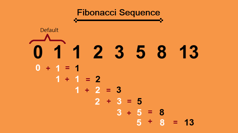
Mathematically, it can be defined by the recurrence relation:
F(n) = F(n-1) + F(n-2)
with initial conditions F(0) = 0 and F(1) = 1
Now this isn’t a math lecture, and hopefully you’re still with me, but the point is that trying to translate this directly into code doesn’t work well.
// Function for getting the number in the sequence at position n
function fib(n: number): number {
  if (n <= 1) return n; // Base case
  return fib(n - 1) + fib(n - 2); // Recursive addition
}
This implementation works, but the issue is that every call to fib(n) (except for the base cases) spawns two more calls: fib(n - 1) and fib(n - 2). Each of those makes two more, and so on, until you hit the base cases. That branching factor of 2, repeated n levels deep, gives you roughly 2ⁿ (technically ≃ 1.618ⁿ) calls in total. With this algorithm, getting fib(100) could take decades to run (assuming the call stack can handle it) because of the astronomical number of branches it must process (≃ 800 quintillion calls).
Let’s compare the recursion trees for fib(5) and fib(8) to see how quickly the call stack can grow.
fib(5)
├── fib(4)
│   ├── fib(3)
│   │   ├── fib(2)
│   │   │   ├── fib(1)
│   │   │   └── fib(0)
│   │   └── fib(1)
│   └── fib(2)
│       ├── fib(1)
│       └── fib(0)
└── fib(3)
    ├── fib(2)
    │   ├── fib(1)
    │   └── fib(0)
    └── fib(1)
fib(5) makes 15 function calls.
fib(8)
├── fib(7)
│   ├── fib(6)
│   │   ├── fib(5)
│   │   │   ├── fib(4)
│   │   │   │   ├── fib(3)
│   │   │   │   │   ├── fib(2)
│   │   │   │   │   │   ├── fib(1)
│   │   │   │   │   │   └── fib(0)
│   │   │   │   │   └── fib(1)
│   │   │   │   └── fib(2)
│   │   │   │       ├── fib(1)
│   │   │   │       └── fib(0)
│   │   │   └── fib(3)
│   │   │       ├── fib(2)
│   │   │       │   ├── fib(1)
│   │   │       │   └── fib(0)
│   │   │       └── fib(1)
│   │   └── fib(4)
│   │       ├── fib(3)
│   │       │   ├── fib(2)
│   │       │   │   ├── fib(1)
│   │       │   │   └── fib(0)
│   │       │   └── fib(1)
│   │       └── fib(2)
│   │           ├── fib(1)
│   │           └── fib(0)
│   └── fib(5)
│       ├── fib(4)
│       │   ├── fib(3)
│       │   │   ├── fib(2)
│       │   │   │   ├── fib(1)
│       │   │   │   └── fib(0)
│       │   │   └── fib(1)
│       │   └── fib(2)
│       │       ├── fib(1)
│       │       └── fib(0)
│       └── fib(3)
│           ├── fib(2)
│           │   ├── fib(1)
│           │   └── fib(0)
│           └── fib(1)
└── fib(6)
    ├── fib(5)
    │   ├── fib(4)
    │   │   ├── fib(3)
    │   │   │   ├── fib(2)
    │   │   │   │   ├── fib(1)
    │   │   │   │   └── fib(0)
    │   │   │   └── fib(1)
    │   │   └── fib(2)
    │   │       ├── fib(1)
    │   │       └── fib(0)
    │   └── fib(3)
    │       ├── fib(2)
    │       │   ├── fib(1)
    │       │   └── fib(0)
    │       └── fib(1)
    └── fib(4)
        ├── fib(3)
        │   ├── fib(2)
        │   │   ├── fib(1)
        │   │   └── fib(0)
        │   └── fib(1)
        └── fib(2)
            ├── fib(1)
            └── fib(0)
While fib(8) makes 67 calls. You can imagine how many calls fib(20) would make.
You may notice that many of these calls repeat; for example, when calculating fib(8), fib(4) is called five times, even though it returns the same result each time.
This shows that exponential algorithms should be treated like a plague to be avoided at all costs, as they don’t scale well. There are other better methods for implementing the Fibonacci sequence algorithm:
- Memoization — If you prefer to stick with the recursive function approach, you can store previously computed values so each function is only executed once. (This can be your take-home or take-to-AI assignment).
- Tabulation — This approach involves building the answer iteratively from the bottom up, capitalizing on the fact that we already know the first two numbers in the sequence. I prefer this method because it allows you to return the entire sequence in an array, not just the number at the specific position you’re looking for. (Another assignment)
By now, you might be thinking that algorithms using recursion are bad, but that’s not exactly true — recursion itself isn’t the issue. What made fib exponential wasn’t the fact that it called itself, but that each call spawned two more calls, with neither reusing the work the other had done. A recursive function that calls itself only once per step and avoids repeating work can be perfectly efficient.
Let’s consider this algorithm that calculates the factorial of a number
function factorial(n: number): number {
  if (n <= 1) return 1;
  return n * factorial(n - 1);
}
Each call to factorial(n) makes exactly one more call to factorial(n — 1). For example, factorial(5) calls factorial(4), which then calls factorial(3), continuing down to factorial(1). It’s a single chain of n links, making the algorithm O(n), with no branching and no repeated work.
Some common exponential operations:
- Generating every possible subset (the power set) of a set.
- Solving the traveling salesman problem by brute-force checking every route.
- Brute-force password cracker.
7. O(n!) — Factorial Time
Algorithms in this category evaluate every possible permutation of the input. This results in factorial growth, which surpasses exponential complexity because each additional step multiplies the total by an ever-increasing factor. This algorithm is so terrible and rare that it’s not worth considering.
Consider this example:
function permute(arr: number[]): number[][] {
  if (arr.length <= 1) return [arr];

  const result: number[][] = [];
  for (let i = 0; i < arr.length; i++) {
    const rest = [...arr.slice(0, i), ...arr.slice(i + 1)];
    for (const perm of permute(rest)) {
      result.push([arr[i], ...perm]);
    }
  }
  return result;
}
To build every arrangement of n items, you pick any of the n items to go first, then any of the remaining n - 1 to go second, then any of the remaining n - 2 to go third, and so on down to 1. Multiply those choices together — n × (n-1) × (n-2) × ... × 1 — and that's n! by definition. It's not an approximation like 2ⁿ; the number of permutations of n items literally is n!.
The growth here is extreme. With 5 items, you get 120 permutations — no big deal. But 10 items jumps to 3.6 million, and 15 items skyrockets past a trillion. Once you hit around 20 items, generating every permutation becomes impossible to wait for, no matter how fast your machine is.
Other places this shows up:
- The traveling salesman problem, solved by brute force — checking every possible order to visit a set of cities.
- Generating all permutations of a list, like anagram generators trying every letter arrangement.
- Brute-force solving a puzzle where you need to test every possible sequence, like scheduling
ntasks in every possible order to find the best one.
Whenever you find yourself writing "try every ordering of the input," stop and look for a smarter approach. Factorial growth (n!) is plain terrible; even a small input of 20 items will exceed practical time limits. Instead, try other methods like dynamic programming, pruning, or heuristics to handle complexity efficiently.
Conclusion
We’ve gone from O(1), where input size hardly matters, to O(n!), where it matters so much that even small inputs become unmanageable. The real takeaway is that Big O isn’t about memorizing a handful of categories — it’s about learning to look at code and ask: as the input grows, does the work stay constant, increase gradually, or explode out of control?
A good habit to build is evaluating loops and recursive calls in relation to input size rather than just counting them. A loop that runs a fixed number of times remains constant regardless of input growth, while one that scales with the input increases complexity. Similarly, a recursive function that executes a single call per step is different from one that branches into multiple calls. These distinctions are precisely what separate linear growth from quadratic or exponential complexity.
It’s important to remember that Big O isn’t the only factor when picking an algorithm. A well-crafted O(n²) approach can beat a poorly implemented O(n log n) one on small, fixed-size inputs when constant factors and overhead are considered. Big O shows how performance scales, not which is faster in your specific case, especially with small inputs. Use it to spot algorithms that won’t hold up as data grows, but don’t treat it as the sole measure of good code.
Understanding algorithmic complexity is far more than an academic exercise; it is the foundation of sound engineering decisions. It determines whether you opt for a hash map over a linear scan, implement memoization for recursion, or recognize when a nested loop will buckle as your dataset grows. Identifying inefficient growth patterns early is a minor adjustment; addressing them once your application scales to a million users is a significantly more difficult and costly conversation.
Comments
Loading comments…