Learn to Build a Neural Network From Scratch — Yes, Really.

In this massive 76 minute tutorial, we’re going to build a neural network from scratch and understand all the math along the way.

I’ve made this guide free because it’s what my younger self would have wanted.

This article is meant for all kinds of people. Whether you’re interested in machine learning yet never coded a day in your life, a seasoned expert in deep learning yet never got down to the nitty gritty, or even a parrot — ok, maybe not that one — today you’ll finally learn to build a neural network.

Building a neural network from scratch is the one coding exercise that makes you 100% better as a developer or engineer of any kind for these three reasons:

• You become more familiar with difficult math.
• You understand how deep learning works on a deep (excuse the pun) level.
• You understand how to make code more efficient using vectorization.

I’m assuming you’re a total beginner, so this will be a long, long tutorial.

The only prerequisite you need is to be able to solve the equation below because I don’t have an eternity to explain all of Algebra.

But anyway, feel free to skip to any sections you care about and skip the fundamental sections marked below if you already have some machine learning (ML) knowledge.

• Fundamentals: What is machine learning?%20What%20is%20machine%20learning%3F)
• Fundamentals: Crash course on matrices%20Crash%20Course%20on%20Matrices)
• Fundamentals: Crash course on derivatives
• Fundamentals: Crash course on partial derivatives
• The perceptron model%20The%20perceptron%20model)
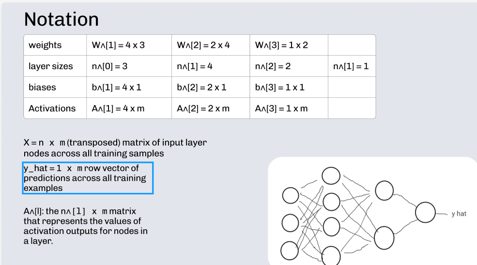
• Basic neural network notation%20Neural%20Network%20Notation)
• Feed Forward%20Feed%20Forward)
• Vectorization%20Vectorize%2C%20Vectorize%2C%20Vectorize)
• Cost%20Cost)
• Backpropagation%20Backprop)
• Build that network%20Build%20that%20network)
• Bonus: How neural networks work
• Bonus: How ChatGPT works

Throughout this article, I’ll point you to external resources if you want to learn more about a given subject, because all I’m giving you is the barebone essentials. I’ve excluded everything that although is helpful, is unnecessary to build a strong neural network intuition.

Read this article with this mindset:

The code is not important. The concepts and math are.

1) What is machine learning?

Have you ever wondered how ChatGPT seems like it’s able to understand you? Or how if you show a picture of a snake to Gemini, it can classify what kind of snake it is?

Despite how seemingly human machines are, and how it would be impossible to fake that sort of knowledge, that is exactly what machines do — they fake it ‘till they make it.

Think back to when you were a dumb baby who didn’t know anything about anything. You learned how to classify people, animals, trees, etc., but how?

If you were born into a white family, the only people you interacted with were your parents. You must have thought all people were white, until you saw other living things. They had the same features as your parents, but had brown, black, or yellowish skin.

They didn’t look like dogs, cats, or zebras. You had to expand your definition of human to encapsulate more and more people — short, tall, skinny, fat, with or without legs. You expanded your knowledge because you got more data.

In a nutshell, that is exactly how a machine also learns. If you give a computer a picture of Jerry Seinfeld and classify him as a human being, the computer will think that Jerry Seinfeld is the *only *human that exists in the world. It will fail to classify any other person as a human being.

But if you give the machine a picture of 100,000 human beings, telling each time “this is a human, this is a human,” then the computer will construct a broader definition for what a human looks like — face, arms, around 5 to 6 feet tall, wearing clothes, different skin colors, etc.

Machines learn from data, just like humans do. The more data a machine has, the more its “worldview” and knowledge expands.

Of course, the quality of the data matters. If you grow up telling a child that every banana they see is actually an apple, whenever they point to a banana, they’ll truly believe in their mind that the long yellow fruit is actually called an apple.

How would a fellow classmate of this unfortunate child correct that behavior? Well, they would tell the kid, “dude, that’s a banana.” Correct that misguided spawn enough times, and eventually he’ll learn the correct names for bananas and apples.

So what happened here? **The child learned from his mistakes and errors and corrected them. **Again, exactly like a machine learns.

Machine learning consists of these steps:

• Gather **correctly labeled **data for the machine to train on.
• Create a metric to describe how much error the machine makes when trying to predict what something is.
• Iteratively train to reduce that error.

Cost intuition

When you first use a machine for machine learning, the predictions it makes are utter trash. So we “punish” the model just like how we “punish” a child by telling them that they’re wrong. But for machines, we take it one step further — we tell them *how *wrong they are, which we call the **cost **of the model.

Let’s say we train a model to classify cats and dogs, and we test it by giving three images of dogs. It instead classifies all of them as cats.

So how many did it get right?

It got 0/3 right, so it obviously did pretty bad. But 1/3 is a better a score than 0/3, and 2/3 even more so. We can quantify the rate of errors through cost, with a basic implementation as follows:

Cost = number of errors / number of total predictions

So in the case of our super trash model, out of 3 predictions it made 3 wrong guesses, so the cost = 3/3 = 1, which is the highest cost for the model.

All machine learning consists of is trying to minimize this cost metric as much as possible. A cost of 0 means we get 0 wrong predictions out of a total 3 predictions (0/3), which makes our model get everything right.

Just understand this: Low cost = good model, high cost = bad model

You can think of cost as synonymous to a grade — you get a D in a class, you don’t really know the material, but if you get an A, you’re doing swell.

But how do we actually minimize this cost? That’s where the complicated math comes in, and we’ll learn that soon.

Right now, let’s draw an analogy to neural networks. As the name implies, neural networks are trying to copy what the human brain does in hopes of creating artificial intelligence on par with that of humanity.

A human brain has 100 billion neurons, so a machine model of the human brain (a neural network) will have 100 billion computing thingies, which we’ll call parameters for simplicity.

If the cost if a measure of how poorly a model is doing, then it needs the output of the model first, which needs the 100 billion parameters to compute the final output. This makes the cost a behemoth of a function, taking in 100 billion variables and outputting a single number.

Can you even minimize let alone understand a function of that size? Can you minimize the cost by hand? Here are the answers to both questions respectively:

You can. You can’t — that’s why we use computers.

Machine learning summary

So now you know what machine learning is. When trying to get a machine learning model to classify stuff like images or data, we tell it what the right answers are and we test it on the data.

From that testing, we get a cost metric for how poorly the model predicts stuff, and we do an iterative process involving complicated math to minimize that cost.

When the cost is minimized, that means the model is predicting stuff correctly, almost as well as a human.

2) Crash Course on Matrices

Matrices are a concise way to represent systems of equations. When you have to crunch several hundreds of numbers together (as you often have to do in machine learning), matrices are the key to making everything comprehensible.

For example, how would you represent (2 * 1) + (3 * 5) + (2 * 2) concisely? Like so:

Here we are multiplying two vectors (I’ll explain later) together in an operation called the dot product, which happens in these steps:

• For the first element in the first vector, multiply it with the first element in the second vector.
• For the second element in the first vector, multiply it with the second element in the second vector.
• For the third element in the first vector, multiply it with the third element in the second vector.
• Now sum up those three numbers, and that’s the dot product.

You pair up each element from both vectors in order, multiply them, and then add up those resultant numbers, so let’s go through the math:

• First pair: 2*1
• Second pair: 3*5
• Third pair: 2*2

Added all up together, you get 2 + 15 + 4 = 21. So when you dot product two vectors together, you get back a single sum, which we call a scalar.

Keep in mind you cannot dot product two vectors together if they have different lengths. What if one vector has 2 elements and the second vector has three elements? That third element in the second vector has no other element to pair up with, and thus blows up and fries your calculator (ok, not that dramatic).

Vectors are one dimensional matrices, meaning they act just like a list of numbers.

To gain a deep understanding about vectors, look at the following video (not needed to build a network, but extremely helpful):

[Embedded content](Learn about what vectors represent here)

Matrices are more complicated. They are 2-dimensional, and can have many rows and columns. Here is an example of a matrix:

So let’s review terminology:

• When you think of a scalar, think of a single number.
• When you think of a vector, think of a list of numbers.
• When you think of a matrix, think of a table of numbers.

Why do we care so much about matrices? Because matrix multiplication can turn a lot of number crunching into simple expressions. For example, what if I want to solve many equations at once?

In the example below, we’re solving 4 equations, resulting in 4 sums total.

Matrix multiplication works as follows:

• In the first matrix, take the first row of the first matrix (see how it’s a vector because it’s one dimension, just a list of numbers) and the first column of the second matrix (also a vector!) and dot product them together. That’s the first entry of the resultant matrix. This is the (25 + 37) calculation.
• In the first matrix, take the first row of the first matrix and the second column of the second matrix and dot product them together. That’s the second entry of the resultant matrix. This is the **(26 + 38)** calculation.
• In the first matrix, take the second row of the first matrix and the first column of the second matrix and dot product them together. That’s the third entry of the resultant matrix. This is the **(15+ 47) calculation.
• In the first matrix, take the … are you even listening anymore?

Yeah, I get it. Matrix multiplication is exhausting and honestly confusing. The good new is that you don’t have to understand how to do matrix multiplication, only when it’s possible.

The most important factor of matrix multiplication is understanding the dimensionality behind each matrix and how the resultant matrix is going to look like.

If you learn nothing else from this article, at least learn this next section:

Matrix multiplication dimensionality

If a matrix has 2 rows and 2 columns, it is a 2 x 2 matrix (read the “x” as “by”).

If a matrix has 3 rows and 4 columns, it is a 3 x 4 matrix.

So the general formula for describing the dimensionality of a matrix is rows x columns, always. This notation matters for understanding which combination of matrices we can and can’t multiply.

Two matrices can be multiplied together if the first matrix has dimensions a x b, and the second matrix has dimensions b x c, and then the resultant matrix will have dimensions a x c.

What do I mean by this? Well, the number of columns in the first matrix has to be exactly equal to the number of rows in the second matrix.

Let’s try out a matrix multiplication combination that cannot get downright funky and multiply:

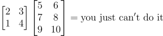
If we try to do the dot product between the first row of the first matrix, and the first column of the second matrix, you can see that 9 is all by its lonesome. Who do we pair it up and multiply it with — the void? See, you can’t do it.

The general rule you might have caught on to is that the rows in the first matrix must have the same size (same number of elements) as the columns in the second matrix. You can’t dot product two vectors if they have different sizes.

What if we switched these two matrices around?

Now the multiplying dimensions correctly follow the **a x b **and the **b x c **pattern, producing a resultant **a x c **matrix. Let’s walk through the dimensions:

• **a: **The number of rows in the first matrix, which is 3
• **b: **The number of columns in the first matrix, which is 2
• **c: **The number of columns in the second matrix, which 2

So a **3 **x 2 matrix times a 2 x **2 **matrix produces a **3 x 2 **matrix. I like to think of this operation as sort of “smashing” and merging the middle two numbers together, like so:

• 3 x 2 times 2 x 2
• 3 x 2ohnoimgettingsmashed2 x 2
• resultant matrix dimensions: 3 x 2

Let’s do another example for reinforcement.

• 4 x 8 times 8 x 3
• 4 x 8ohnoimgettingsmashed8 x 3
• **resultant matrix dimensions: **4 x 3

One last final tip to note is that when multiplying matrices, order matters. Here is an example where we multiply two 2 x 2 matrices together (so their dimensions will always be valid), but we do it in two different orders and get wildly different results.

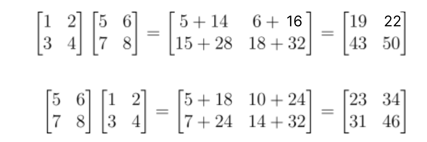
In the context of machine learning, the order in which to multiply matrices can be very confusing, but as you’ll see later down the line, the most important part is just getting the dimensions to match. This non-commutative property of matrix multiplication is important to keep in mind, but you won’t have to deal with it.

Great. Now that you know how matrix dimensions work, there is one last step to master before you will have learned all the linear algebra you need to create a neural network.

For a more detailed understanding, watch these two great videos:

Transposition

Transposition is a simple concept. You transpose a matrix by just switching around its rows and columns.

In the below example, we transpose a 3 x 2 matrix into a 2 x 3 matrix. The “T” symbol just means we are transposing the matrix.

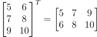
The first column of the matrix becomes the first row in the new transposed matrix.

The second column of the matrix becomes the second row in the new transposed matrix, and this pattern continues.

Why is transposition important? Because it lets us multiply two matrices together that we otherwise couldn’t have.

Let’s go back to the previous example:

But what if we transpose that 3 x 2 matrix into a 2 x 3 matrix?

Transposition allows us to multiply two matrices together without changing the order (which as you learned before, order matters).

Matrix transposition also gives us great flexibility in matrix multiplication according to this law:

Why don’t you try to prove it yourself? Use these matrices below.

Summary

• A dot product between two vectors returns a single number.
• For matrix multiplication, order matters.
• You can only multiply two matrices if the first matrix has dimensions a x b, and the second has dimensions b x c, resulting in a matrix with dimensions a x c.
• Transposing a matrix swaps its columns and rows. It makes a matrix with dimensions **a x b **turn into a matrix with dimensions b x a.

Derivatives

Calculus is the secret sauce that lets us minimize the cost function we talked about earlier. Yes, you read that right — the cost of a machine learning model is just a math function.

We’ll go into details later, but understand that the cost function is huge, taking in thousands of variables as an input. To minimize the cost, we need to find out its slope so we can figure out which direction to head in.

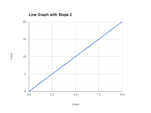
Derivatives are a way to find the slope of any function. If you look at the line graph below, we can tell it has a slope of 2 (remember rise over run?).

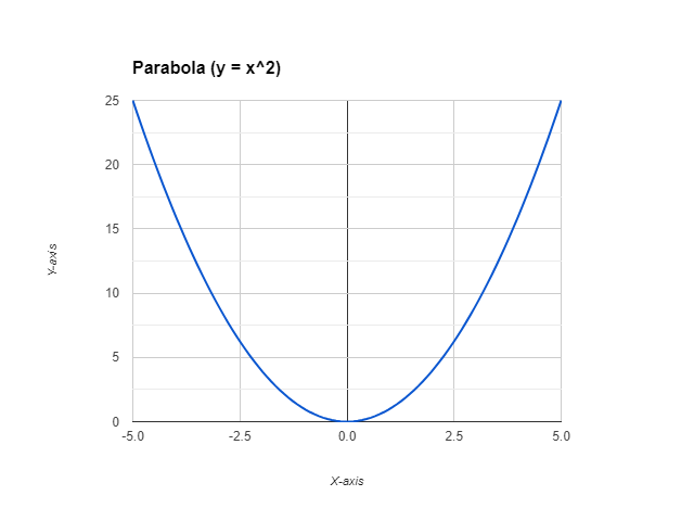
But how can we find the slope of a more complex function like a parabola? That’s where derivatives come in.

Usually a whole semester of calculus goes into teaching what derivatives are and how to calculate them, but I’ll keep it brief.

Explaining what a derivative is

Let’s go back to the parabola example from earlier: it’s not a line, so there’s no rise over run. You may think calculating the slope of a parabola is impossible, but look closer — a lot closer.

Zoom in far enough on one section of a parabola, say x = 3.0 to x = 3.001 and it will appear as a straight line. Now *that *you can calculate the slope of.

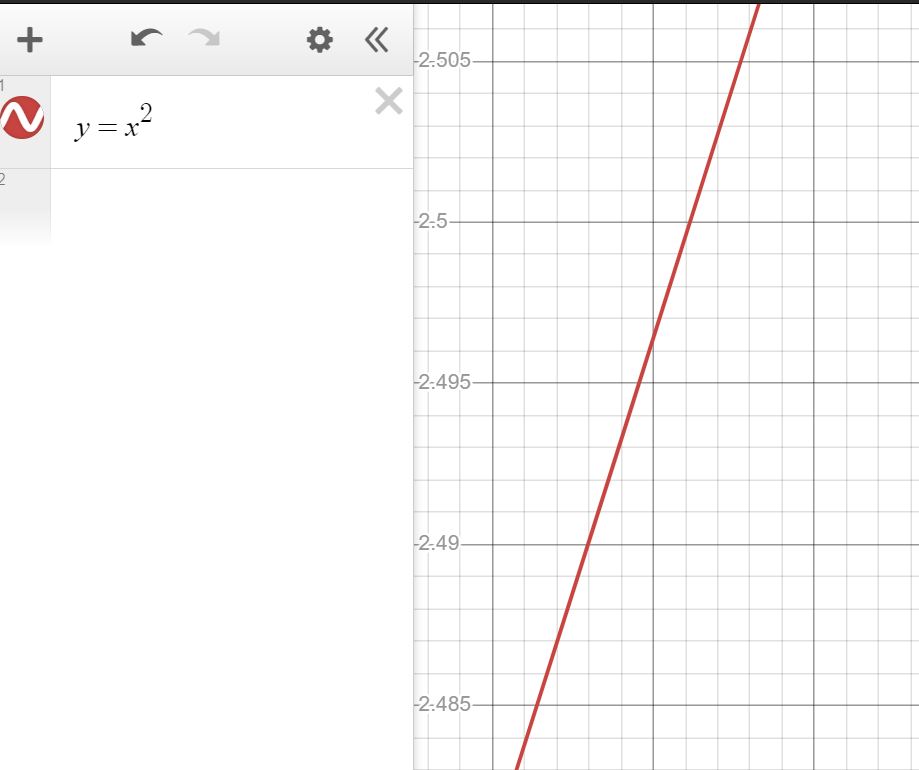
This same concept of zooming in applies to all functions ever created. Zoom in enough, and that section becomes a line you can get the slope of.

However, there is a catch: the slope changes depending on where you are in the graph. It’s not static like it is for a line. The slope between x = 3.0 to x = 3.001 is different than x = 1.0 to 1.001.

That is what a derivative is — the algebraic equation that represents the slope of the graph at all points on the graph.

For a parabola, the derivative would be an algebraic equation representing the line y = 2x. You can also think of the derivative as the algebraic equation tangent (perpendicular) to the graph at all points.

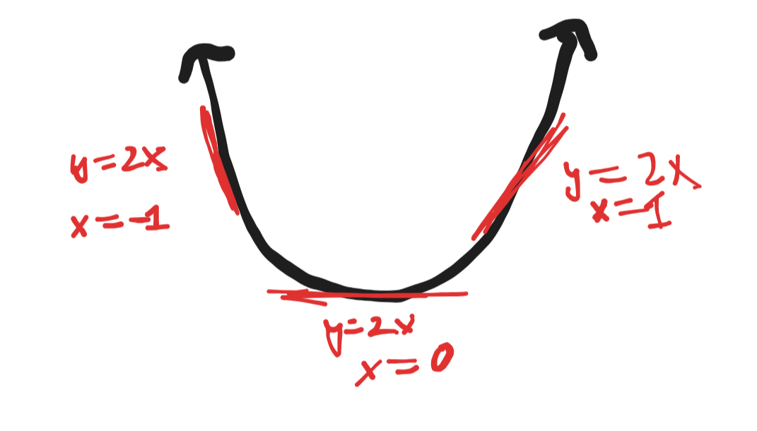
If you still don’t understand, don’t worry. All you need to know is how to calculate derivatives.

Calculating derivatives: Power rule

How did we find the derivative of y=x² earlier? Well let’s use the power rule:

• Slip down the exponent of x² — the 2 — down in front and multiply it against the base, giving you 2x²
• Subtract one from the exponent, giving you 2x¹
• Smile in joy with your final result = 2x.

Let’s try to find the derivative of y = 3x²:

• Slip down the 2, giving you (3 * 2)x² = 6x²
• Subtract 1 from the exponent giving you 6x¹ = 6x.

For a more succinct notation, we swap out y for f(x) because it’s better to think in terms of functions for machine learning.

So if f(x) = 4x², we represent the derivative of f(x) with the notation f’(x) — called f prime of x — is f’(x) = 8x.

Ok, let’s get into when the power rule isn’t so obvious.

How would you find f’(x) for f(x) = 2x? The power rule still applies.

• The exponent on the x term is 1, so slip the 1 down, giving you (2 * 1)x¹
• Subtract 1 from the exponent, giving you 2x⁰. Then realize anything in the world to the 0th power is just equal to 1, which gets you 2 * 1 = 2.

So if f(x) = 2x, the derivative f’(x) = 2, which was just the constant multiplying x. So for any f(x) = cx, where c is a constant, then f’(x) = c. This makes intuitive sense:

We represent a line with a slope equal to 2 as y = 2x, and what else is the derivative other than the slope of a function? The derivative here is just equal to the slope, which is f’(x) = 2.

And the final case to think about is the derivative of a constant. We can’t use the power rule to find the derivative of a constant like f(x) = 5, but I’ll just fast forward to the answer:

For all f(x) = c where c is some constant real number, f’(x) = 0. So the derivative of any constant is 0. This makes intuitive sense:

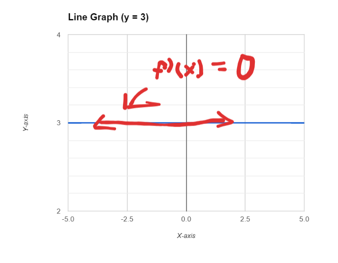
The line f(x) = c where c is a constant just represents a flat line. Take for example f(x) = 3. It’s a flat line, which means no rise and all run, giving a slope = 0. Thus it makes sense for the derivative f’(x) to equal 0.

Calculating derivatives: Multiple terms

If f(x) = x + 5, how do we find f’(x)? Well the rule is simple: just find the derivative of each individual term.

The derivative of x is 1, and the derivative of the constant 5 is 0, so we get f’(x) = 1.

If f(x) = 2x² — 3x + 8, the derivative is just 4x-3 + 0 = 4x-3.

Calculating derivatives: Product rule

Let’s say that we are multiplying two functions f(x) and g(x) together as h(x) = f(x)g(x) and we want to find the derivative of that.

Here is the general formula:

h’(x) = f’(x)g(x) + f(x)g’(x)

Before you rush to the nearest cliff and try to jump off it, hear me out — let’s work through an example.

• f(x) = 3x, g(x) = 2x²
• so the derivatives are f’(x) = 3, g’(x) = 4x
• This leads to h’(x) = 3(2x²) + 3x(4x) = 6x² + 12x² = 18x²

Let’s prove that this works by multiplying f(x) and g(x) together and then taking the derivative:

• f(x) * g(x) = 6x³
• The derivative of 6x³ is 18x², so we proved it!

If you want to understand why this works and how people found out about it, me too. But we’re already 20 minutes in and we haven’t talked about neural networks at all.

Let’s move on.

Calculating derivatives: Summation

Building on the same idea of how the derivative of a sum is just the derivatives of each individual part, all summed together, we can do the same thing with summations.

How would we find f’(x) for this?

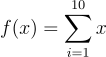
You could just do the sum first and then take the derivative, which would get you f(x) = 10x, which makes f’(x) = 10. Let’s think a bit smarter.

Since the summation just sums up all the terms, we can just use the derivative sum rule to take the derivative of all the individual parts of those sums, *and then *sum them all up.

So the first step is to find the derivative of x, which is 1. Then we just sum up those ones.

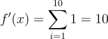
Calculating derivatives: Chain rule

The chain rule is by far the most essential parts of learning derivatives. You may not understand anything at all, and going over the intuition would require me to teach you about limits, secant lines, etc., so we’re only going to learn *how *to do the chain rule.

I highly recommend watching this video if you have the time to build up an intuition beyond “yeah bro, just f prime of x that.”

The chain rule is concerned with finding derivatives when functions are composed, like f(g(x)). How would you find the derivative of that? This is what the chain rule says:

If h(x) = f(g(x)), then h’(x) = f’(g(x)) * g’(x)

First let’s do it the old fashioned way with f(x) = 4x² and g(x) = 3x³.

• f(g(x)) = f(3x³) = 4(3x³)² = 4(9x⁶) = 36x⁶.
• The derivative of 36x⁶ is — frantically searches up 36 times 6 — 216x⁵.

Now let’s do it with chain rule:

• f’(g(x)) = f’(3x³) * g’(x) = f’(3x³) * 9x²
• To find out what f’(3x³) is, we first need to find f’(x).
• f’(x) = 8x, so f’(3x³) = 8*3x³ = 24x³.
• So f’(3x³) * 9x² = 24x³ * 9x² = 216x⁵.

Great, we proved it! Now it’s time to learn notation that we will use for machine learning.

We can rewrite the chain rule as follows:

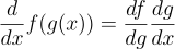
The d/dx syntax just means taking the derivative of an equation with respect to x. It’s another way of rewriting f’(x). For example, d/dx of 2x is just the derivative of 2x, which equals 2.

This notation is important because it showcases a chain, something you can’t do the f prime notation.

Let’s break it down:

• d/dx f(g(x)) means we are trying to find out f’(g(x)), just like chain rule.
• df/dg is a succinct way to write out df(x)/dg(x), meaning that we want to find out the derivative of f(x) with respect to g(x), which we write out as f’(g(x)).
• dg/dx is our old friend g’(x).

So let’s go back and do the calculations with f(x) = 4x² and g(x) = 3x³.

• **df/dg: **f’(g(x)), and f’(x) = 8x which equals f’(3x³) = 8(3x³) = 24x³
• **dg/dx: **g’(x) = 9x²

We then multiply these two terms together to arrive at the answer once again: 216x⁵.

One useful feature of this notation is the illustration of a chain, especially if you think about fraction multiplication. This may be too confusing to think about for now, so we’ll tackle this again when we talk about partial derivatives.

Calculating derivatives: Special derivatives

There are a few special derivatives that you should know how to calculate since they will be used in the backpropagation calculations. All of these use chain rule.

If f(x) = ln(x), which is the natural log of x, then f’(x) = 1/x * 1 = 1/x. It’s just 1 over whatever was on the inside, and then because of chain rule, you multiply by the derivative of the inside term.

Let’s do another example, but keep in mind chain rule: If f(x) = ln(2x²), then f’(x) = (1/2x²) * 4x = 2/x. We multiplied by 4x because that is the derivative of 2x².

Ok, this one is really weird — if f(x) = e^x, then f’(x) = e^x. It’s just the same thing.

But with chain rule, if f(x) = e^{2x}, then f’(x) = e^{2x}*2 = 2e^{2x}. We multiply by the derivative of 2x which is just 2 because of the chain rule.

Fundamentals: Partial Derivatives

Congratulations, this is the last piece of fundamental math knowledge you need before you can build a neural network from scratch.

If we have a function that lives in three dimensions like z = 2x + 3y, how can we find the slope of that? Trick question — you can’t.

But we can fake it. You can get the derivative of a multidimensional function with respect to one variable at a time, treating all other variables as constants.

This is called a partial derivative, where we treat only one variable in a multivariable equation as an actual variable, and everything else as a constant.

If a function f takes in two variables x and y, like f(x, y), we can represent the partial derivative of f with respect to x as ∂f/∂x (pronounced “del f del x”).

How can we calculate ∂f/∂x if f(x, y) = 2x + 3y?

• Since we are trying to find the partial derivative of f with respect to x, we treat x as a variable and y as a const.
• What is the derivative of 2x while treating x as a variable? It’s just 2.
• What is the derivative of 3y while treating y as a constant? Well 3 times a constant is still a constant, and the derivative of any constant is equal to 0.
• We arrive at ∂f/∂x = 2 + 0 = 2

Let’s try to find ∂f/∂y if f(x, y) = 2x + 3y.

• Treat y as the variable here and x as the constant.
• ∂f/∂y = 0 + 3 = 3.

Gradient descent intuition

The intuition behind partial derivatives is to think about how a single variable in a multidimensional function affects the output of that function. ∂f/∂x asks, “if I only change x and keep all other variables constant, how does that change in x affect the output of my function f?”.

That is the most important question in machine learning.

What if I could find the partial derivative of my machine learning model’s cost with respect to a single variable? Then I could tweak that variable accordingly to minimize the cost as much as possible.

I’ll reiterate: Calculus is the secret sauce behind how a machine learns. Partial derivatives allow us to find how any variable affects the cost of a model and tweak it accordingly to make the cost smaller or larger at our will.

If ∂f/∂x is positive, like say ∂f/∂x = 2, then it translates to, “if x increases by some small value, then the function f increases by that small value times 2.”

If ∂f/∂x is negative, like say ∂f/∂x = -2, then it translates to, “if x increases by some small value, then the function f decreases by that small value times 2.”

Let’s say the cost function of the model has some variable/parameter called w. If ∂C/∂w is positive, that means if w increases, then the cost C also increases. So let’s do something smart — let’s decrease the value of w. If w decreases, then so will C.

I’ll let you work out for yourself whether we should increase or decrease w to minimize the cost if ∂C/∂w is negative.

This is the heart of machine learning — gradient descent. Let’s say that our cost function C has 1000 variables, named w_1, w_2, etc., making it a whopping 1000-dimensional function. We notate C as C(w_1, w_2, …, w_n)

The gradient of C is denoted as ∇C, which is just the collection of all the partial derivatives of C with respect to each one of its 1000 variables:

Looks familiar? It’s just a vector. The partial derivative of cost with respect to its first variable, ∂C/∂w_1 becomes the first entry, and then so on until ∂C/∂w_1000.

The gradient gives us mastery over the once beastly cost function — we now know how tweaking each variable changes the cost function.

You can think of each partial derivative as a dial, where turning it left decreasing it) or right (increasing it) adjusts the cost accordingly. With the power of machine learning, you now have a thousand dials to tweak at your will, allowing you to omnisciently change the cost.

But no human can manage 1000 dials, let alone 100 billion that a typical neural network has. Instead, we make the network figure it out.

If a machine learning model has ∇C, it knows exactly how each dial changes the cost and how much to turn each of them.

For example, if ∂C/∂w_1 = 1 and ∂C/∂w_2 = 9, then we can see that ∂C/∂w_2 has a bigger effect on the cost function. You increase the variable w_2 by 1 unit, and the cost C will increase by 9!

Thus the knob ∂C/∂w_2 gives us the biggest bang for our buck in terms of changing the cost.

If this explanation didn’t stick, I’d encourage you to reread it. Partial derivatives underly the entire intuition behind how neural networks work.

Chain rule with partial derivatives

I promise that this is the last piece of math we need before we can fully understand neural networks.

Chain rule with partial derivatives builds on the normal chain rule idea. It’s hard to explain, but easy to show.

Let’s say I have a function v = 3x + 4y, x = 3a², and y = 4b². How can I get ∂v/∂a or ∂v/∂b if I’m dealing with composed functions nested within each other?

You could try substituting in x in terms of a and y in terms of b to directly calculate ∂v/∂a and ∂v/∂b, but what if v was more complicated, like 3x⁵+4y²?

Then substituting in x = 3a² and y = 4b² into v, you would end up with v = 9a¹⁰ + 64b⁴, which is a lot more messier than working with each equation separately.

The chain rule simplifies calculations with complex algebraic expressions by tackling them piecemeal.

Let’s build a computation graph:

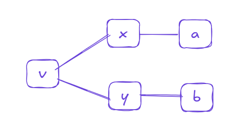
The function v is made up of the variables x and y, and x is made up of a, and y is made up of b. This tree is the single most helpful diagram to draw out before computing any partial derivatives.

If I want to find ∂v/∂a, I need to travel from v to x, giving me ∂v/∂x, and then from x to a, giving me ∂x/∂a. You then multiply them together to create the chain rule:

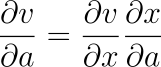
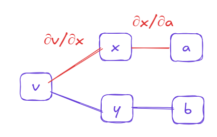
Another way that makes sense is the idea of fraction multiplication. Although you are not dealing with fractions at all, you can kind of see how the denominator of ∂v/∂x and the numerator of ∂x/∂a are the same — ∂x — and therefore “cancel out”.

That is the **chain, **my personal method of choice for calculating partial derivatives. The chain and the tree are the easiest way to calculate these essential derivatives.

Let’s try another one: what’s ∂v/∂b?

First we use the chain and tree to construct what the partial derivative calculation should look like:

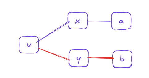
• Construct the chain: ∂v/∂b = (∂v/∂y) * (∂y/∂b)
• Calculate ∂v/∂y: v = 3x + 4y, so ∂v/∂y treats y as a variable and everything else as a constant, therefore ∂v/∂y = 0 + 4(1) = 4
• Calculate ∂y/∂b: y = 4b², so ∂y/∂b treats b as a variable and everything else as a constant, therefore ∂v/∂y = 8b
• **Multiply the chain together: **∂v/∂b = 4(8b) = 32b

Once you get used to the notation, you realize calculus isn’t so hard after all. If you understand the chain and tree method, and are able to do these calculations, you’re in a great spot to build your own neural network.

5) The perceptron model

It only took 15 years and 3 high school graduations — congrats to your kids by the way — to get here, but you made it.

A neural network is roughly modeled after a human neuron. A neuron takes in an input, does something, and returns an output. I don’t know — I’m not a biologist.

But neurons connect to other neurons, which in turn feed input to even more neurons.

So following that biological intuition, we represent networks as a collection of a bunch of nodes.

• Each node has a numeric value.
• We connect nodes to other nodes using weights, which work as multipliers to values.

It’s easier to just show you:

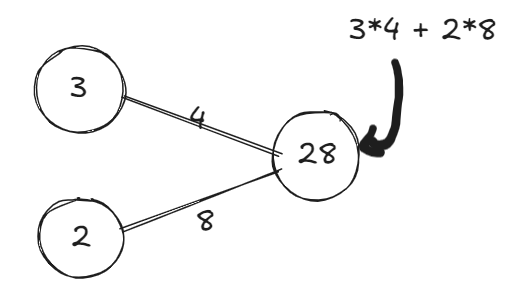
In this first layer, we have two nodes. We observe three things:

• The first node’s value = 3 and the second node’s value = 2.
• The first node has a weight = 4 connecting it to the node in the second layer.
• The second node has a weight = 8 connecting it to the node in the second layer.

For the node in the 2nd layer, how did I know that the value was 28?

To get the value of a node that is being connected to from nodes in the previous layer, you basically sum up the node value times the connecting weight, for all nodes connecting to that node.

I know, it’s kind of hard to explain — so I’ll just show you:

• First node has value 3, with weight 4. Multiply the node and weight value together, and the product is 12.
• Second node has value 2, with weight 8. Multiply the node and weight value together, and the product is 16.
• Add these two products together, and you get 12 + 16 = 28.

Does it look familiar? It’s a dot product between the values of a node and the weights connecting them to a node in the next layer:

So a layer in a network has four rules:

• Each node in a layer must connect to every single other node in the next layer using connections called weights.
• Every weight has a predetermined value that we choose randomly. We don’t know the values of nodes.
• Only the first layer of nodes starts out having values, usually called the input layer.
• Every other layer of nodes gets calculated based on the previous layer and weights connecting them.

TLDR: we choose the weights for each layer and the inputs to the network, and from those two things we can calculate the values of all nodes in the network.

Let’s move on to a bigger example:

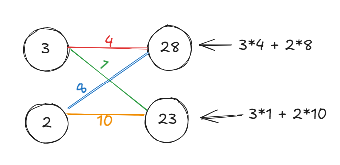
Since each node in a layer must connect to each other node in the next layer, we end up with 2 x 2 = 4 weights. Let’s expand this to other sizes:

• **3 nodes in first layer, 5 nodes in second layer: **Each node in the first layer has to connect to each node in the second layer, and there are 5 nodes in the second layer, so that is 5 weights per node in the first layer. Since there are 3 nodes in the first layer, you get 3 x 5 = 15 weights.
• **i nodes in first layer, j nodes in second layer: **You end up with i times j = ij number of weights.

The first node in the second layer got the value of 28 because it was connected to the red weight and blue weight.

• The red weight = 4, and connects to a node with value 3, giving it the product 12.
• The blue weight = 8, and connects to a node with value 2, giving it the product 16.
• Add these two products together and you get 28.

The second node in the second layer got the value of 23 because it was connected to the green weight and yellow weight.

• The green weight = 1, and connects to a node with value 3, giving it the product 3.
• The yellow weight = 10, and connects to a node with value 2, giving it the product 20.
• Add these two products together and you get 23.

Biases

The last thing we need before we can move onto notation is the idea of a bias.

A bias is a number added to a node’s value at the end of the weight dot product calculation. Here are the two rules for using biases:

• We apply biases to each node except for the nodes in the input layer.
• Every node (besides those in the input layer) has their own randomly assigned bias of our choosing.

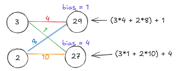
In the example above, we give each node in the second layer its own bias value, and add that after the weight calculation.

A bias is important because if each of our weights were 0, then the resulting neuron values for the second layer would always be 0. The famous disease of 0 would propagate throughout each layer, until the entire network just computes 0.

A bias avoids that by adding a value at the end of each neuron calculation, unaffected by multiplication with 0.

So here are the rules of biases:

• Each node has its own randomly assigned bias value, except for nodes in the input layer.
• Biases are added the value of a node after the weight multiplication thing.

That first rule is important and has intuition behind it. Imagine if in the split second you see a fox and your brain tries to classify that brownish blob as a fox rather than some amalgamation of color, your brain decides, “damn bro, let me add a tiara and jacket onto that thing before processing it.”

We see the world as raw input, not as biased input.

Neural Network Intuition

Weights, nodes, biases … what? I agree that it’s confusing, but remember those dials I talked about earlier in the partial derivatives section?

Weights and biases are the **dials **we can control to get a desired output.

We don’t have control over the first layer since that is the raw input (think of your brain classifying a fox — you don’t get to decide *how *to classify it), and we don’t have control over any nodes in the network since those are always determined by the node values in the layer before it.

The only stuff we can control are those weights and biases, the trusty knobs and dials that only our computer has the power and speed to operate.

What do we as humans know? Well, we know how bad a neural network did in trying to predict something. Once a neural network runs some input through its network, we as humans decide how bad the network did by mathematically designing some cost function that quantifies the difference between network’s output and the expected, correct output:

• If the cost is low for a test input, the network is good.
• If the cost is high for a test input, the network is bad.

And if the output was bad, resulting in a high cost? Well, all is not lost.

The computer knows every single number in a network: all the inputs, weights, and biases that led to the output. We can then use calculus to see how much each weight and bias contributed to that bad output.

The insight? — this allows us to update each weight and bias precisely as to reduce the cost.

So our neural network will compute a cost function C that includes all those weights and biases, and it can learn how to update those weights and biases accordingly to minimize the cost through the gradient ∇C.

Summary

Neural networks have these 4 components to them: nodes, weights, biases, and cost.

Here are the steps of running a neural network:

• You provide the input data to the network as the input layer, and then network uses that values from the input layer and the weights connecting it to the second layer to compute the values for the second layer.
• This process propagates through all layers of the network, until each node in the network has a value.
• The last layer will output the network’s prediction, which we then compare to our labeled data to provide a cost metric for the network.
• Based on the cost, we can calculate the gradient with respect to cost ∇C and update the weights and biases accordingly.
• Repeat steps 1–4 until we minimize the cost as much as possible.

Here are the rules of neural networks you should keep in mind:

• For a node in a layer, it’s connected to every single node in the next layer through connections called weights.
• Weights are randomly initialized to begin with, but we change them based on the gradient ∇C.
• Every node in the network — except for the nodes in the input layer — have a bias, which is added to the node after the weight-node multiplication. The initial values for the biases don’t matter — just assign them randomly.

We can now move on to basic neural network notation:

6) Neural Network Notation

The secret behind understanding neural networks is to have the correct notation. If you have too many indices and nodes flying around, combining to form the Lochness monster of equations, even the most seasoned ML expert will cower in fear.

Simplicity is key. Everything will make sense in section 7, which is where I’ll teach you the true intuition behind neural networks.

Before that, however, we have to learn notation.

Layers of a network

Think of the standard image of a brain: you think of a neurons connecting to other neurons for miles and miles, not a giant wall of neurons linked side by side.

Neural network layers are based on the same premise. We have three types of layers:

• **input layer: **This is the first layer in a neural network, but it’s also not really a layer. We think of the input layer as the raw *input *to the model, not actually part of the neural network itself.
• **hidden layers: **All layers in between the input layer and output layer are called hidden layers. As the name implies, we don’t have any intuitive way to describe what they do behind the scenes. We can only interpret what the input layer means — raw input — and what the output layer means —the network’s output. The hidden layers? They’re just pure computation.
• **output layer: **The last layer is the output layer, which should output the prediction of the network.

We can architect a network to solve any problem possible. For example, what if we want to predict if a person is at risk for cardiovascular disease solely based off their weight and height? Here are the numbers:

• **input layer: **We take in two inputs — a person’s weight and height — so our input layer will have *two *nodes.
• **hidden layer: **As many nodes and layers as we want. Sky’s the limit.
• **output layer: **There are only two possibilities — the person is at risk for cardiovascular disease or not at risk — which means we can encode that with a single probability output. 0 for not at risk, and 1 for at risk. The output layer will then have one node, since we only have to output one number.

Here is an example network I created that we’ll use to build up our intuition for the rest of the section:

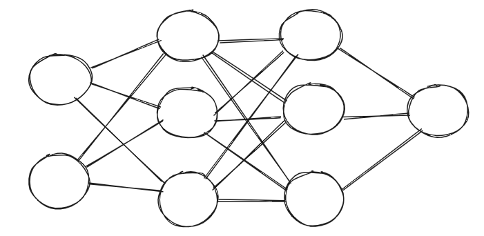
When working with layers, it’s essential to number each layer and know how many nodes each layer has.

We count layers starting at the first hidden layer, excluding the input layer (it’s raw input so it doesn’t count).

However, we will also count the input layer as the 0th layer sometimes, since it makes the math and notation easier. Just understand the convention is to always label the first hidden layer as the 1st layer of the network.

In the above network, we have two hidden layers and one output layer, so we have **3 **layers total.

We represent the total amount of layers in the network using the variable L, and here L=3.

For counting nodes, we represent the number of nodes in each layer with n⁽ˡ⁾, where l is the layer number. For this, you can optionally include the input layer, which we would represent with 0.

Let’s write out all the layer size notations for n⁽ˡ⁾ for all layer numbers:

Quick question — what’s n⁽ᴸ⁾?

Well L is the total number of layers in our network (excluding input layer), which is 3, so L=3. Then n⁽ᴸ⁾ = n⁽³⁾ = 1, which makes sense because we have 1 node in the output layer.

Weights

Let’s zoom in on a small portion of our network, just the input layer and first hidden layer.

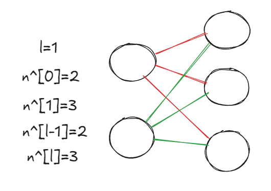
The number of nodes in the input layer (0th layer) is n⁽⁰⁾ = 2, and the number of nodes in the first hidden layer (1st layer) is n⁽¹⁾ = 3.

We want to find some succinct way to represent the set of weights that connect the current layer (layer 1) to the previous layer (layer 0), but how can we do that? Is there a pattern?

Let’s walk through our thinking:

• Each node in the 0th layer connects to every node in the 1st layer.
• There are three nodes in the 1st layer, so each node in the 0th layer has 3 connections.
• There are 2 nodes in the 0th layer, so we have 3*2 = 6 connections, meaning there are 6 weights total.

We found out how many weights there are in between the 0th and 1st layers, but we can expand that for any layer.

For any layer l, there will always be n⁽ˡ⁾ ⋅ n⁽ˡ ⁻ ¹⁾ weights connecting layer l-1 to l.

Here l=1, so n^[l] = 3 (number of nodes in layer 1), and n^[l-1] = 2 (number of nodes in layer 0). We get 3*2 = 6 weights, just like before.

Why does this matter? Well if you can remember from last time, finding the value of a node in the next layer took a lot of calculations:

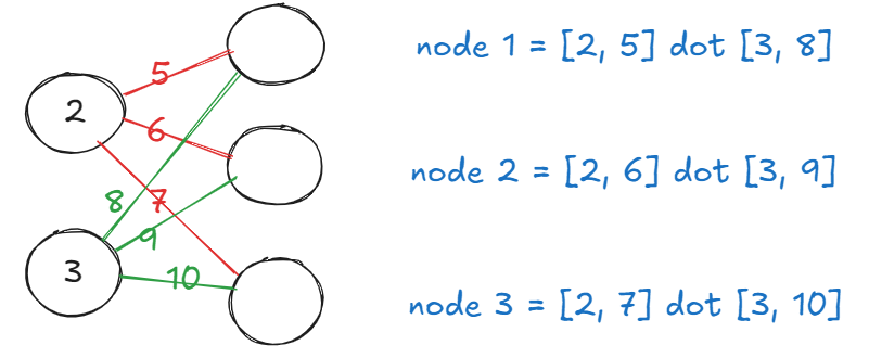
It’s easy to get lost in the forest of dot products, so let’s try an easier way: matrix multiplication.

Here is our goal:

• Represent each layer of the network as a matrix (reshaped from a vector).
• Represent each set of weights in between two layers as a matrix.

First let’s build intuition:

• Gather all the red weights and place them in a vector: [5, 6, 7]
• Gather all the green weights and place them in a vector: [8, 9, 10]
• Notice how we can represent the nodes in 0th layer as a 2 x 1 matrix (2 rows, 1 column), which is pretty much the same thing as a vector.
• Notice how we can represent the nodes in 1st layer as a 3 x 1 matrix (3 rows, 1 column), which is pretty much the same thing as a vector.

Aren’t the node values just a list of numbers? Why not use a vector? While we could do that, using matrices makes the math for matrix multiplication easier. A vector and a matrix with a single column or single row are essentially equivalent, but representing the layers as matrices will be much more valuable in the future once we lay out all the math.

Let’s introduce new terminology:

• **row vector: **A vector with n elements reshaped to be a matrix with a single row, having dimensions 1 × n.
• **column vector: **A vector with n elements reshaped to be a matrix with a single column, having dimensions n × 1.

By reshaping any layer of nodes to be row vectors and column vectors (which are 2-dimensional matrices) instead of just leaving them as 1D vectors, the math works out in our favor.

After all, why deal with 16 different vectors when you can deal with 2 matrices instead?

So we want to create a matrix multiplication equation that multiplies a 2 x 1 matrix by the matrix of weights and then results in a 3 x 1 matrix.

Let’s try it out:

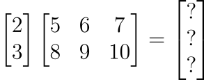
Silly us — our dimensions are wrong! You can’t multiply a 2 x 1 matrix by a 2 x 3 matrix since the middle dimensions don’t match up.

Let’s try again via the transposing the column vector to be a row vector instead.

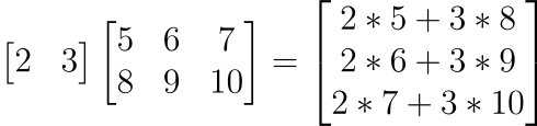
Ok, so this works. Notice how we got the exact same answers a minute ago when we did the dot product manually, but now we have a concise representation of all the node values in the 1st layer.

Although this is a perfectly fine solution (and a lot better than the dot products), we will take it one step further to make building neural networks even easier.

Let’s transpose the weights matrix and make it the first matrix in the matrix multiplication.

But wait, doesn’t order matter? Yes, but in this particular case, via the law of transposition, we still produce the exact same calculations and solution so we’re fine.

Remember that if you have two matrices M₁ and M₂ and then you multiply them together, then the law of transposition states the following: (M₁M₂)ᵀ = M₂ᵀ M₁ᵀ

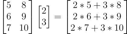
Now that we represented our weight matrix as a 3 x 2 matrix, we can extrapolate that process for any layer.

• The 0th layer has 2 nodes, and since the 1st layer has 3 nodes, each node in the 0th layer has 3 weight connections.
• We treat the set of weight connections belong to a node in the 0th layer as a vector of size 3, since there are 3 connections.
• There are two nodes in the 0th layer, so we have 2 sets of weights.
• To form the weight matrix, we stack the vectors side by side vertically, so each vector is its own column. This gives us a 3 x 2 matrix.

Now we can describe the dimensions of the weight matrix for any layer l connecting the previous layer l-1.

W^[l] has dimensions n^[l] x n^[l-1] if n^[l] is the number of nodes in layer l and n^[l-1] is the number of numbers in the previous layer l-1.

Layer 1 has 3 nodes and layer 0 has 2 nodes, so the dimension will be 3 x 2. Simple, right?

Using that formula, we can find the dimensions of all the weights in the network:

• W^[1] : 3 x 2 matrix, derived from dimensions n⁽¹⁾ × n⁽⁰⁾
• W^[2] : 3 x 3 matrix, derived from dimensions n⁽²⁾ × n⁽¹⁾
• W^[3] : 1 x 3 matrix, derived from dimensions n⁽³⁾ × n⁽²⁾

Biases

Biases are even simpler than weights. Since each neuron in a layer — except for the input layer — will have a bias, the matrix of biases for a layer will just be the exact same size as a layer itself.

Let’s go back to the 0th and 1st layers:

The nodes in the input layer will not have any biases, but every node in the 1st layer will have biases. There are three nodes in the 1st layer, so there are three biases.

Just like how we represented the 1st layer as a 3 x 1 matrix, the biases in the first layer will also be a 3 x 1 matrix.

In general, we follow this rule to find the dimensions of the biases in a layer:

For any layer l, the bias column vector matrix b^[l] has dimensions n⁽ˡ⁾ × 1.

We now have all the building blocks we need to understand how neural networks compute an output in the feed-forward process:

Summary

It’s really important that you master the notation before we move on, so I’ll give a quick review:

• **column vector: **We can reshape a vector with n elements to be a column vector, resulting in a matrix with dimensions n × 1. Visualize the vector standing up vertically.
• **row vector: **We can reshape a vector with n elements to be a row vector, resulting in a matrix with dimensions 1 × n. Visualize the vector lying down horizontally.

Here are the three types of layers in a neural network:

• **input layer: **Denoted as the 0th layer. It is the only layer without biases, and has no weights connecting it.
• **hidden layers: **All layers sandwiched in between the input and output layers.
• **output layer: **The last layer in the network. The calculated node values of this final layer are considered as the network’s final output.

Given that a network has L layers (not including the input layer), we can denote the number of nodes in each layer as such:

• n⁽⁰⁾: number of nodes in the input layer
• n⁽¹⁾: number of nodes in the 1st hidden layer
• n⁽ˡ⁾: number of nodes in the lth hidden layer
• n⁽ᴸ⁻¹⁾: number of nodes in the last hidden layer
• n⁽ᴸ⁾: number of nodes in the output layer

The hidden layers comprise all layers indexed 1 to L-1, and the output layer is indexed as layer L.

We represent all nodes in a layer and all biases in a layer as column vectors, and we represent all weights between two layers as a matrix.

• **nodes: **For a layer l, you represent the nodes for that layer as a column vector with dimensions n⁽ˡ⁾ × 1.
• **biases: **For a layer l (excluding the input layer) you represent the biases for that layer as a column vector with dimensions n⁽ˡ⁾ × 1, since each node has its own bias.
• **weights: **The weights matrix connecting layer l-1 to layer l will have dimensions *n^[l] x n^[l-1]*.

7) Feed Forward

Feed forward is the idea of calculating all node values for each layer, continuing until you reach the final layer and calculate the final output.

Consider the final output to just be the calculate values of the nodes in the last layer: the output layer.

However, to calculate the output layer, we need to calculate all the previous hidden layers. In a nutshell, that is feed forward.

There’s almost nothing new here — we just have to generalize the process.

The feed forward process

The best way to understand feed forward is to just do it. We already did some of it, but I left a lot of it out.

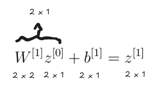
Let’s go back to this example, but now to generalize feed forward we need to describe this mathematical process using our beloved neural network notation:

For now, let’s represent the column vector matrix of nodes in a layer as z^[l] for some layer l.

Let’s write out what we know:

• z^[0] : the 2 x 1 matrix of elements [3, 2], representing the 0th layer.
• z^[1] : the 2 x 1 matrix representing the 1st layer.
• W^[1]: the 2 x 2 matrix representing the weights connecting the 1st layer and 0th layer.
• b^[1]: the 2 x 1 matrix of elements [1, 4], representing the biases for the 1st layer.

Now we’ll use notation to describe the calculations instead of numbers:

• We matrix-multiply the weights W⁽¹⁾ by the nodes in the input layer, z⁽⁰⁾.
• For each node in the 1st layer, add their respective biases. This is the same as just overall adding the column vector b⁽¹⁾.

Just so we can double check our math, here are the calculations:

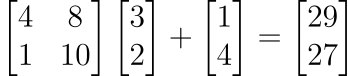
We arrive at the same answer, so we know our formula is correct. Let’s put in words:

To get the values for the nodes in the next layer, we need to matrix multiply the weight matrix by the node values from the previous layer, and then add the bias values to the result.

Are we done? Not quite…

Activation functions

I omitted a step from the feed-forward process, but we’ll get to it now. Once we get a value for the neuron with the weight matrix multiplication and bias addition, we need to squish that value down into something our networks can deal with.

**activation functions **do this modification. There are two important attributes an activation function must have:

• Must be nonlinear, as in it CANNOT be in the form g(z) = mz + b.
• Must compress the input to a predetermined range, like 0 to 1.

The intuition behind these two requirements?

Unimportant but nice intuition: Well, if the activation function were nonlinear, the best thing our neural network could do is simple linear regression. Essentially, it would just be a giant, sophisticated line of best fit predictor. We need nonlinearity to model complex functions.

The activation function we will be using is the *sigmoid *function, which looks like so:

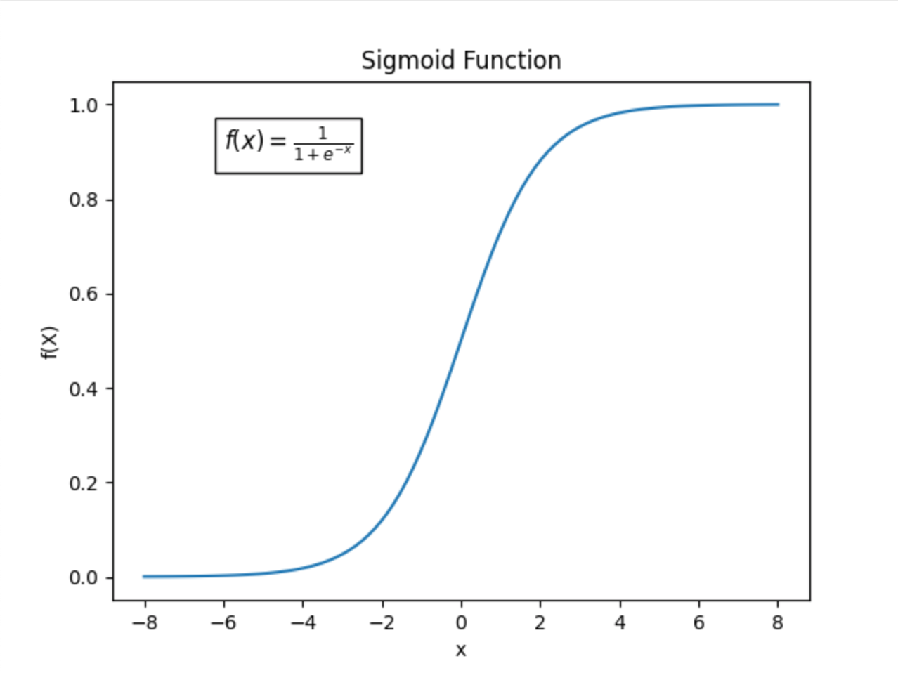
We will use this equation because it most closely models how a real neuron works: they are either on or off, but also have a small transition window that’s kind of a half-on half-off thing.

A note for the future: the convention is to notate the activation function as g(z).

The sigmoid function ranges between 0 and 1. As you go to the right, the sigmoid function output flatlines at 1, and as you go to the left, the sigmoid function output flatlines at 0.

Now that we know what an activation function is, we can go back to our network from before:

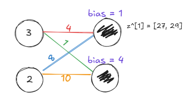
The z^[1] calculation is just an intermediary step, where the first node in layer 1 has value 27, and the second node in layer 1 has value 29.

Now we pass those z values into our sigmoid activation function g(z) = 1/(1 + e⁻ᶻ) to get back the actual values for nodes in a layer, which we’ll denote as a^[l].

When we pass in 27 into g(z), we get g(27) = 0.99. For 29 into g(z), we get g(29) = 0.99.

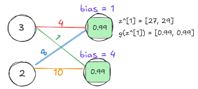
Now we can actually represent the 1st layer as it truly is: a^[1] = [0.99, 0.99].

Essentially, we’re following these steps:

• Calculate z⁽ˡ⁾, which we can consider as our unprocessed output.
• Calculate a⁽ˡ⁾, which we can consider as plugging in z⁽ˡ⁾ into our choice of activation function (sigmoid) to get the final processed output a⁽ˡ⁾, which represents the final values of nodes in a layer l.

Let’s put these calculations into a formula:

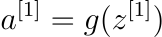
So the feed forward process has these steps:

• Matrix multiply the weight matrix by the activations of the previous layer, and then add the bias matrix of the current layer. This gives you the pre-activated node values for a layer l, z^[l].
• Pass in the pre-activated layer z^[l] into sigmoid activation function g(z) to get a^[l]. This represents the final values of nodes in a layer.

Before we completely generalize for any layer l, we have to talk about inputs and outputs.

Inputs and outputs

Going back to the tenets of machine learning, we need data for a machine to learn — lots of it.

Returning to the cardiovascular disease example, we fed our network two inputs — their height and weight. What if we have 10,000 rows in a database, each representing a person’s height and weight? We’d have a 10,000 x 2 matrix of input data. We would call each person a training sample, and since we have records of 10,000 people, we have 10,000 training samples.

We notate the matrix of input data as X.

We also have a database of 10,000 rows, corresponding to the same people, each with a number that’s either 0 or 1.

0 if they are not at risk for cardiovascular disease, and 1 if they are. This is what we want for our output data.

**We notate the matrix of output data as Y. **Since the output data was a 1 dimensional vector, it’s better to make it a column vector matrix since that makes the math easier.

This is machine learning in a nutshell — we provide the inputs and outputs so the neural network can learn the patterns, and then generalize to new inputs that nobody knows the answers to.

Why is this important? Because we’ll make X as the input layer for our network, giving our network feeding in the entire training data.

But we’ll get to that later once we talk about vectorization. Right now, let’s pick one person to be our only training sample — Jimmy, who weights 150 pounds and is 70 inches tall.

We represent Jimmy the training sample as X^[i] for the ith training sample, which we will represent as X^[i] = [150, 70]

Since we will use this training sample as the input to our network, and we know we can also call the input layer the 0th layer, we don’t we designate the input [150, 70] as a^[0]?

Here is what our network will look like:

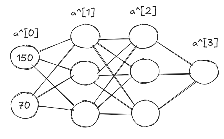
Let’s do the calculations for layer 1 and make sure our dimensions match:

• a^[0] is our input layer with dimensions 2 x 1 since the input layer has 2 nodes.
• a^[1] is the 1st layer activations with dimensions 3 x 1 since layer 1 has 3 nodes.
• W^[1] is our weight matrix layer with dimensions n^[1] x n^[0] = 3 x 2.
• b^[1] is the bias matrix for layer 1 with dimensions 3 x 1 since the first layer has 3 nodes.

Here are the equations, which should be very familiar by now.

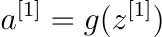
The great thing about the way we set up our notation is that we don’t actually have to check our math. As long as the matrix dimensions are correct and multiply correctly, we can be 99% sure our math is doing it’s thing.

One last time, let’s walk through the dimensions:

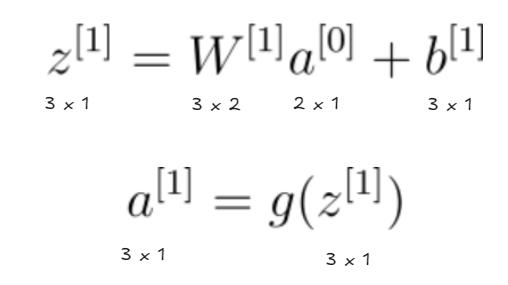
Yup, it all works out. Now it’s time to stop holding your hand. You’ve probably already noticed the feed-forward pattern already, but I’ll generalize it so you can do the rest of the matrix math yourself.

For any layer l, the following is the feed forward process for a neural network:

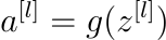
• Exercise: as an exercise, try to represent a^[2] and a^[3] as algebraic expressions using this feed forward process.

Once you get to the last layer L=3, you’ll get the final output of the network: a^[L].

The output

Note that all nodes in the network will have a value between 0 and 1 because of the sigmoid activation function, which allows us to model probability.

In machine learning, we notate the output of a machine learning model in a special way: ŷ (pronounced “y hat”).

ŷ represents the prediction of the network, and we compare ŷ to y (the true values we’re the testing the model on) to create an error metric for the model that measures how poorly the network predicts the stuff we want.

Let’s go back to Jimmy: what if the network predicts that Jimmy the training sample [150, 70] has a 0.72 probability of being at risk at cardiovascular disease, but it turns out Jimmy’s true diagnosis is that he’s not at risk for cardiovascular disease.

So when we compare our predicted value ŷ = 0.72 (72% probability of being at risk for cardiovascular disease) to y = 0 (no risk of cardiovascular disease), then the cost for our model is (predicted-expected), which equals 0.72.

This simplistic cost model has the highest possible cost being 1 (completely wrong) and the lowest possible cost as 0 (completely write).

Getting a cost of 0 means that our predicted value ŷ should be exactly equal to y, which means the cost ŷ-y = 0, which is what we want.

Before we write the code for the feed forward process, let’s talk it through:

• Randomly initialize the weights and biases for the network.
• Do the feed forward process for each training sample.
• Get the ŷ at the end of the feed forward process for each training sample.
• Come up with a cost metric for the network across all training samples.

Wait, that sounds like a lot of work.

You’re right, and if you do it this way by looping through all the training examples I guarantee you will end up more confused than were before you even started reading this article.

The final step before we can become neural network wizards is to **vectorize **the entire process across all training examples.

8) Vectorize, Vectorize, Vectorize

This will be a quick but important section. You now have all the intuition to do feed forward by yourself, but I haven’t told you about how to really calculate cost for the network yet.

Cost calculations are only easy if we can vectorize across all training samples first.

Let’s revisit the 10,000 records of height and weight data. The matrix of training input data we called X had dimensions 10,000 x 2.

Vectorizing our training data means that instead of looping and doing the feed forward process for all training samples, we do the feed forward on all the training data at once.

To make the future math easier, we transpose X into a 2 x 10,000 matrix, or more commonly referred to as n x m, where n is the number of features and m is the number of training samples.

What do we mean by features? You can think of it as the number of variables we feed into the network.

• Our network takes in the height and weight of person to predict whether or not they are at risk of cardiovascular disease.
• Height and weight are the two variables we use an input for the network, so we call them our two features.

Wait, two features? Isn’t that the same number of nodes we have in the input layer?

Exactly. Features, input layer, X — all interchangeable. So it’s a bit confusing to say X is an n x m matrix, when n^[0] x m is much easier to understand.

So the input to our network is no longer a column vector with dimensions n⁽⁰⁾ × 1. Rather, we’ll represent it as many input layers at once using the input matrix X with dimensions n⁽⁰⁾ × m.

Spoiler alert: all our intermediary values and activation layers will vectorize across all the training samples as well, and we’ll modify the notation as follows:

• X : the n^[0] x m matrix of training data. The same thing as the input layer.
• A^[0]: the same thing as X, just notated differently to be compatible with the 0th layer alternate definition for the input layer.

In general, we will represent the vectorized layer of activations across all training samples for a layer l as A^[l]. These vectorized activation layers will always have m (number of training samples) columns, and their number of rows is equal to the number of nodes in that layer, n^[l].

Sidenote: Although we’re always technically dealing with matrices, we only notate a matrix with a capital letter if it has more than one column, as in it can’t be shaped into a vector. So now our activations

We don’t vectorize the weights and biases of our network because we only want one copy of the weights and biases to generalize for all training samples. So we’re good on that front.

Let’s revisit the math, keeping in mind the following:

• n^[0] : 2
• n^[1] : 3

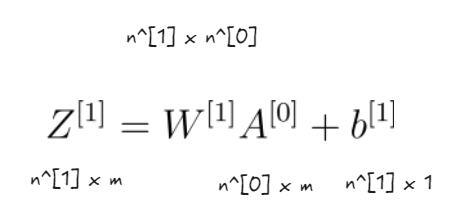
• We multiply the weights matrix of dimensions 3 x 2 by the vectorized input layer of dimensions 2 x m to get a 3 x m matrix as a result.
• It’s impossible to add a 3 x 1 matrix and a 3 x m matrix together. The bias matrix is 3 x 1, but we need to stretch it to have dimensions 3 x m by copying it over and over m times. This process is called broadcasting. Then we can just add two 3 x m matrices together to get Z^[1] as a 3 x m matrix.

And for the final activation output?

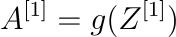
Well we know that both Z^[1] and A^[1] have the same dimensions, so this is fairly easy.

So much of neural networks comes down to just getting the matrix dimensions right. With vectorization you can rely on matrix multiplication rather than complicated loops.

Let’s expand this for any layer l:

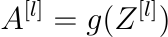
• Z^[l] : pre-activation values for layer l, vectorized across all training samples. Has dimensions n^[l] x m.
• A^[l] : post-activation node values for layer l, vectorized across all training samples. Has dimensions n^[l] x m.
• A^[l-1] : node values for layer l-1, vectorized across all training samples. Has dimensions n^[l-1] x m.
• W^[l]: matrix of weights between layer l-1 to l, with dimensions n⁽ˡ⁾ × n⁽ˡ⁻¹⁾.

Let’s see if you can calculate the dimensions for A^[2] and A^[3] on your own.

The code

Here we are.

Before you shed a tear, stop and suck it back in. Tears aren’t good for coding.

If you don’t care about the code, you can skip ahead to the backpropagation section. You have already learned everything you need to know for feed forward — at this point it’s just practice.

You can also follow along and run the code yourself here:

[NN From Scratch

• *An interactive python notebook to run the neural net example from scratch — colab.research.google.c](https://colab.research.google.com/drive/1rLdJzcpwpf6Tq36frEbPuiqN4TIkf5q5?usp=sharing)om

But anyway, let’s get started:

The Code: The Phantom Menace

The first step is to decide on our network architecture. Let’s go back to our cardiovascular disease example:

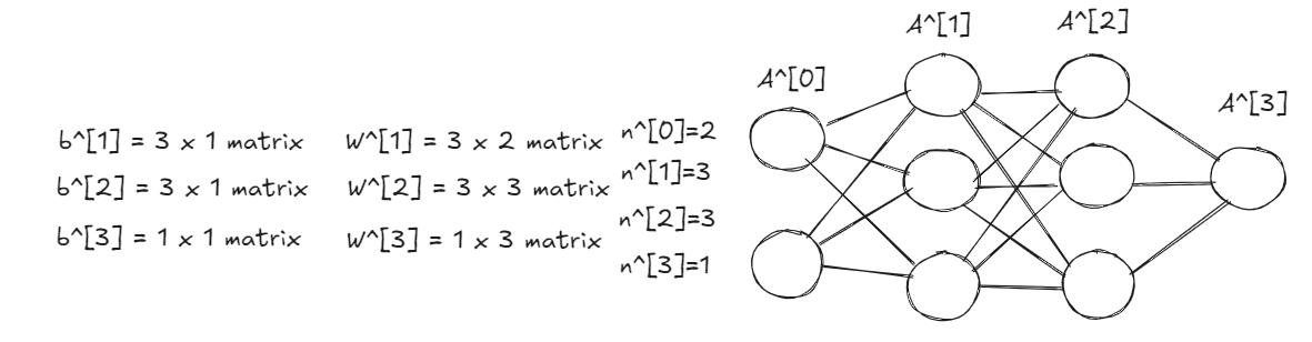
Given an n^[0] x m matrix of training data called X, we want to feed the input forward through the network until we arrive at a final output A^[L]which has dimensions n^[L] x m. We call this final output as ŷ, the neural network’s prediction.

Here is the architecture in code:

n = [2, 3, 3, 1]
print("layer 0 / input layer size", n[0])
print("layer 1 size", n[1])
print("layer 2 size", n[2])
print("layer 3 size", n[3])

When I say n=[...], with those square brackets it means I’m creating a list in Python. You can think of a list in Python exactly like a vector, but you can’t do math with it.

If we create a python array with arr=[10,20,30], you can get the first item in the list by writing arr[0], then the second with arr[1], and so on. It’s a bit confusing, but makes sense with the neural network layer notation we set up earlier with n^[0], etc.

The Code: Attack of the Clones

Now we need to randomly initialize the biases and weights.

We can do this using the numpy library from python, and then creating a matrix with random values using the np.random.randn() method.

import numpy as np

W1 = np.random.randn(n[1], n[0])
W2 = np.random.randn(n[2], n[1])
W3 = np.random.randn(n[3], n[2])
b1 = np.random.randn(n[1], 1)
b2 = np.random.randn(n[2], 1)
b3 = np.random.randn(n[3], 1)

Here I’m just following the standard formula that for the weight matrix in a layer W^[l], the dimensions should be n[l] x n[l-1]. For the bias matrix in a layer b^[l], the dimensions should be n^[l] x 1.

We can check our shapes by using the .shape property that numpy matrices have:

print("Weights for layer 1 shape:", W1.shape)
print("Weights for layer 2 shape:", W2.shape)
print("Weights for layer 3 shape:", W3.shape)
print("bias for layer 1 shape:", b1.shape)
print("bias for layer 2 shape:", b2.shape)
print("bias for layer 3 shape:", b3.shape)

The above code prints the following text, affirming that our dimensions are correct:

Weights for layer 1 shape: (3, 2)
Weights for layer 2 shape: (3, 3)
Weights for layer 3 shape: (1, 3)
bias for layer 1 shape: (3, 1)
bias for layer 2 shape: (3, 1)
bias for layer 3 shape: (1, 1)

The .shape property for matrices describes the dimensions of the matrix and returns an ordered pair called a tuple, in the form of (rows, columns).

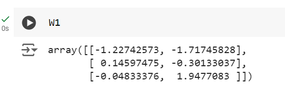
Here is what a numpy matrix looks like:

The Code: Revenge of the Sith

Now that we’ve initialized the weights and biases, let’s prepare our input data X. We know that we want X to be a matrix of a bunch of training samples, where each training sample has two features — height and weight.

But along with X, we need the true labels for the training data. We can’t expect the network to get stuff right if we never give it the correct answers to start with.

X = np.array([
    [150, 70], # it's our boy Jimmy again! 150 pounds, 70 inches tall. 
    [254, 73],
    [312, 68],
    [120, 60],
    [154, 61],
    [212, 65],
    [216, 67],
    [145, 67],
    [184, 64],
    [130, 69]
])

print(X.shape) # prints (10, 2)

Now we have our training data in the shape m x n, but we need to transpose it for our feed forward process.

We can transpose a matrix by calling the .T property on it, which returns that matrix but transposed.

A0 = X.T
print(A0.shape) # prints (2, 10)

Now we have A^[0] in the shape n^[0] x m, which is exactly what we want.

What about the training labels?

Just a reminder that if the final layer output A^[L] has dimensions n^[L] x m, then the expected training labels also need to be of the same dimensions. According to our neural network, the last layer n^[L] = n^[3] = 1, so the training label data Y will have dimensions 1 x m.

y = np.array([
    0,  # whew, thank God Jimmy isn't at risk for cardiovascular disease.
    1,   # damn, this guy wasn't as lucky
    1, # ok, this guy should have seen it coming. 5"8, 312 lbs isn't great.
    0,
    0,
    1,
    1,
    0,
    1,
    0
])
m = 10

# we need to reshape to a n^[3] x m matrix
Y = y.reshape(n[3], m)
Y.shape

The .reshape() method on a matrix allows us to reshape the matrix to any dimensions we want by passing the rows and columns like matrix.reshape(rows, columns). However, we can only reshape when it makes sense to, where if the rows times columns equals the number of elements in the matrix.

In the above example, we create our training label y, but it’s a vector so we reshape into a matrix Y because it has to match the output of our network A^[L].

The Code: A New Hope

The last part before we can start our feed forward is to create our activation function.

We create functions in python using the def keyword, and this function takes in one argument: a matrix. Then the sigmoid function will be applied to each element of the matrix, which is exactly what we want.

def sigmoid(arr):
  return 1 / (1 + np.exp(-1 * arr))

The np.exp() method takes in a matrix, and models the function e^x.

We can check that it works if all our outputs are between 0 and 1.

The Code: The Empire Strikes Back

Now that we have our weights, biases, activation function, input layer, and training labels, we can begin the feed forward process.

m = 10

# layer 1 calculations

Z1 = W1 @ A0 + b1  # the @ means matrix multiplication

assert Z1.shape == (n[1], m) # just checking if shapes are good
A1 = sigmoid(Z1)

# layer 2 calculations
Z2 = W2 @ A1 + b2
assert Z2.shape == (n[2], m)
A2 = sigmoid(Z2)

# layer 3 calculations
Z3 = W3 @ A2 + b3
assert Z3.shape == (n[3], m)
A3 = sigmoid(Z3)

Do you see how simple vectorizing across the training samples makes the code? No no, don’t thank me now — thank me after backprop.

This is the final output:

print(A3.shape) # prints out (1, 10)
y_hat = A3      # y_hat is essentially the prediction of the model

And here is what y_hat looks like:

Let’s interpret this output in a machine learning context:

For each of the 10 people, our network predicted that they all had around a 54–56% probability of being at risk for cardiovascular disease, and if we round up the 0.5 to a 1, it means our model did extremely poorly just predicting everybody as being at risk for cardiovascular disease.

The network only got 5/10 right, which is 50% accuracy. It makes sense, since we initialized the weights and biases randomly — it’s just flipping a coin.

Our network has a long way to go — but I believe, one day it will save the world (or at least get 80% accuracy).

The Code: Return of the Jedi

For those of you who are more adept with coding, here I organize everything into functions:

import numpy as np

# 1. create network architecture
L = 3
n = [2, 3, 3, 1]

# 2. create weights and biases
W1 = np.random.randn(n[1], n[0])
W2 = np.random.randn(n[2], n[1])
W3 = np.random.randn(n[3], n[2])
b1 = np.random.randn(n[1], 1)
b2 = np.random.randn(n[2], 1)
b3 = np.random.randn(n[3], 1)

# 3. create training data and labels
def prepare_data():
  X = np.array([
      [150, 70],
      [254, 73],
      [312, 68],
      [120, 60],
      [154, 61],
      [212, 65],
      [216, 67],
      [145, 67],
      [184, 64],
      [130, 69]
  ])
  y = np.array([0,1,1,0,0,1,1,0,1,0])
  m = 10
  A0 = X.T
  Y = y.reshape(n[L], m)

  return A0, Y

# 4. create activation function
def sigmoid(arr):
  return 1 / (1 + np.exp(-1 * arr))

# 5. create feed forward process
def feed_forward(A0):

  # layer 1 calculations
  Z1 = W1 @ A0 + b1
  A1 = sigmoid(Z1)

  # layer 2 calculations
  Z2 = W2 @ A1 + b2
  A2 = sigmoid(Z2)

  # layer 3 calculations
  Z3 = W3 @ A2 + b3
  A3 = sigmoid(Z3)

  y_hat = A3
  return y_hat

A0, Y = prepare_data()
y_hat = feed_forward(A0)

And here is what y_hat looks like:

9) Cost

Once you learn about how to actually calculate cost for a network, you’ll be a neural networks expert. No, really.

In fact, as soon as you learn about cost I’ll challenge you to derive backpropagation all by yourself because you’ve already learned all the math you need for this section.

But anyway, let’s return to the idea of cost being (predicted-expected). While that works, it kind of breaks for negative values.

There are many different types of cost functions, which I’ll list below:

• **Mean squared error: **For all (predicted-expected) errors, square them and then add them all up.
• **Root Mean squared error: **For all (predicted-expected) errors, square them and then add them all up. Then take the square root of the resultant sum to get your final result.
• **Mean absolute error: **For all (predicted-expected) errors, use the absolute value to make them positive and then add them all up.

These all work well since they fix the problem of negative numbers, but which one do we pick. Trick question — none of them.

*But why? *Rather than just trying to fix the issue of negative numbers — which most cost functions already do — we need to pick a cost function that is easy for the neural network to minimize.

In the graph of a parabola below, where is the minimum point? It’s where the derivative = 0, or at the vertex.

Let’s say the neural network is a blind man trying to descend down a foggy hill. The foggy hill here is any cost function c(x).

The blind man may not be able to see, but he has one handy superpower: the ability to calculate the derivative of the function at any position. This allows him to always find the “bottom” of any hill/function.

In the example below, it’s easy to get to the bottom because there’s only one “bottom” in a sense.

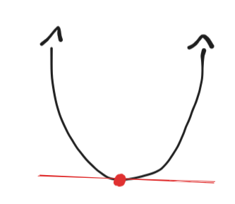
The parabola above has only one minimum, called the global minimum. If a function has only one global minimum, this makes it a **convex **function, which is exactly what we look for in a cost function. Having only one global minimum means that you’re absolutely sure the cost can go as low as possible.

• If the blind man is at position x₀ and he uses his superpower to calculate c’(x₀) > 0 (the derivative of the cost function at position x₀), then he knows he’s currently at an uphill portion (corresponds to the function is increasing). He must therefore go in the opposite direction to go downhill.
• If the blind man is at position x₀ and he uses his superpower to calculate c’(x₀) = 0, then he knows he has reached the bottom, the minimum of the cost function.

What if we were dealing with a non-convex function with many local minima? Then we could get stuck in a local minima, never able to get out again.

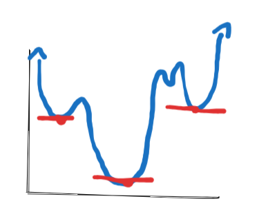
With non-convex cost functions, when trying to minimize the cost, it’s likely that the network will get stuck in a local minimum rather than at the desired global minimum.

This is because the blind man only knows when the derivative of the cost function becomes 0, not the *optimal *point for it. Once he reaches a local minima, he’s happy to stay there.

We’re not happy though. For that reason, we’ll choose a convex cost function.

For classification problems like these, where we want our final output to be between 0 and 1, we’ll use the binary cross entropy loss function, which is **guaranteed **to be convex.

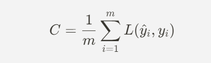
Although these may seem like big scary equations, let’s dissect what they mean:

• yᵢ: the training label output for the iᵗʰ training sample.
• ŷᵢ: the model’s prediction for the iᵗʰ training sample.

L(ŷᵢ, yᵢ) calculates the error for a single training sample and is called the loss function. Let’s dissect this behavior further:

When yᵢ = 0, then the loss function simplifies to ln(1-ŷᵢ), and the following behaviors occur:

• If ŷᵢ = 0, then it simplifies to ln(1) = 0, which means the loss would be 0, and that makes sense. If you predict exactly 0, and the output is also 0, then you got the example right and should have cost = 0.
• If ŷᵢ = 1 or at least approaches 1, then the cost gets exponentially larger ln(0) is infinity.

When yᵢ = 1, then the loss function simplifies to ln(ŷᵢ), and the following behaviors occur:

• If ŷᵢ = 1, then it simplifies to ln(1) = 0, which means the loss would be 0, and that makes sense.
• If ŷᵢ = 0 or at least approaches 0, then the cost gets exponentially larger, since ln(0) is infinity.

The cost function C is just summing up all the losses calculated for all training samples and then averaging them. This is because cost should be an overall metric for how well the network is doing across all training samples.

But as you have may have noticed, calculating the cost and loss requires looping over the training samples. Wasn’t the entire point of vectorization to avoid doing that?

Well we can skip the looping, but it’s a bit hacky:

def cost(y_hat, y):
  """
  y_hat should be a n^L x m matrix
  y should be a n^L x m matrix
  """
  # 1. losses is a n^L x m
  losses = - ( (y * np.log(y_hat)) + (1 - y)*np.log(1 - y_hat) )

  m = y_hat.reshape(-1).shape[0]

  # 2. summing across axis = 1 means we sum across rows, 
  #   making this a n^L x 1 matrix
  summed_losses = (1 / m) * np.sum(losses, axis=1)

  # 3. unnecessary, but useful if working with more than one node
  #   in output layer
  return np.sum(summed_losses)

I wouldn’t expect you to understand this code, but just know that it works. We calculate all the losses at once for each training sample, and then sum them all up and then average them.

If you think the code is scary, don’t be discouraged. As long as you understand the math, you can say you learned how to make a neural network.

We can see what the initial cost our network is:

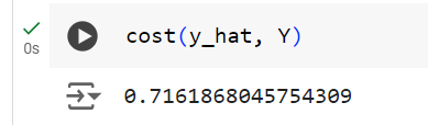
Before backpropagation

Up for a challenge? Then before looking at section 10, derive backpropagation yourself. I promise you if you can do this, you’ll automatically rise to the top 10% of ML practitioners, above the 90% that don’t know any of the math.

As I’ve stated before, machine learning is nothing but computing cost and then trying to minimize it. We can minimize the cost if we know which way to head in.

The gradient of cost is ∇C, which is made up of the partial derivatives of the cost C with respect to all its parameters.

What are the parameters that go into C? Just the weights and biases, so W^l and b^l for all layers in the network starting at l=1.

For our network, ∇C would look something like this:

∇C represents how we should change each parameter to increase the cost as fast as possible. So we should do the opposite of that — head in the direction of the negative of the gradient to decrease the cost as fast as possible.

Now that the laptop knows how to change all the dials/parameters of the network in order to increase or decrease cost, we can reduce the cost.

You know the feed forward process. From that, use the chain and tree method of partial derivatives to find all these partial derivatives.

Here are two tips you need to know before attempting backpropagation on your own:

• Your math is right if the matrix dimensions work. All the partial derivatives have the exact same dimensions as their normal variables. This means that ∂C/∂W^[1] should have the exact same dimensions as W^[1]. For any layer l, ∂C/∂W^[l] will have the same dimensions as W^[l], ∂C/∂b^[l] will have the same dimensions as b^[l], and ∂C/∂A^[l] will have the same dimensions as A^[l]
• After successfully calculating the gradient ∇C, you know which direction to turn those dials, but how much do you turn them? The answer is only a little, since if you turn them a lot you risk overshooting the minimum. When updating the weights matrix W^[1] by ∂C/∂W^[1], multiply that partial derivative calculation first by some small value like 0.01.
• Run the feed forward and backprop steps for at least a thousand since we take small steps each time.

Good luck. If you can manage to do this on your own, you should be immensely proud of yourself.

10) Backprop

This is it. Backpropagation is the beast who defeated many aspiring ML engineers and turned many away from entering the gates of artificial intelligence development.

When I was a junior in high school I failed to tame this beast. But here I am, four years later and ready to teach you the secret behind backpropagation.

Let’s get started.

Intuition

In the previous section, you learned about the best cost function for binary classification tasks:

When do you know you’ve done a good job on a test? Well, when you get 100%. No, let’s go further. When you get all the answers right? Further - it’s when you get no questions wrong.

To make a network learn, to solve any kind of machine learning problem, we need to minimize its cost function C. If our neural network has a cost of 0, it means it got no “questions” wrong in our test analogy, netting it a 100%.

How do we make our cost function as low as possible? We follow these steps:

• Find the slope of the cost function, which we described as ∇C. Use partial derivatives and chain rule to discover this value.
• Update the parameters of the network in the **opposite **direction of the gradient. Take small proportional steps to the gradient.
• Run the above steps again about 10,000 times.

For all the math calculations, we will be using a vectorized approach across all training examples because it makes everything easier to understand. That’s why we used vectorization for the feed forward process as well.

You could find the brightest student at Harvard and teach her backpropagation, but even she would get confused if you throw a bunch of summations and loops around.

Final layer

Ok, so we want to find ∇C. How on earth do we do that?

Well let’s start small — how about we just try to find the gradient of cost with respect to the parameters in the final layer?

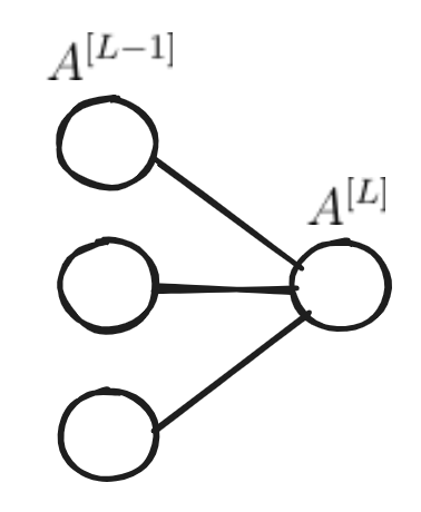
These are the last two layers from the previous cardiovascular disease example.

• The last layer is denoted A^[L] with dimensions 1 x m.
• The second to last layer is denoted A^[L-1] with dimensions 3 x m.
• The weights layer connecting the last layer and second to last layer is W^[L], with dimensions 1 x 3.

Let’s say after a feed forward iteration we calculate A^[L], which let’s us calculate the cost C.

The next big question is this: how do we change the weights in layer L to reduce the cost?

Partial derivatives. Nothing but that. We can describe what we want as ∂C/∂W^[L], which is fancy notation to describe how much each individual weight in W^[L] weights matrix affects the final cost C.

Well, what is C? Remember that we defined the cost of the neural network to be the average of all binary crossentropy losses calculated for each training sample?

So we calculate the cost C like so:

• Sum up all binary crossentropy losses that you calculated for each training sample.
• Average them by dividing the sum by the number of training samples m.

Hmmm… But I don’t see where W^[L] is in the cost function. How could we possibly find the derivative with respect to the weights then?

That’s what the chain rule is for. W^[L] is hidden in the binary crossentropy loss function L. First we need to build a computation graph. Then we can build the tree and visualize the chain of partials to build.

We get the computation graph from the feed forward calculations we did earlier, since that’s the only way you can compute the cost. Backprop is just finding the derivative of all the equations from feed forward.

In the example below, I am doing a few steps that should be obvious, but I’m just explaining as a disclaimer:

• I expanded the loss function L directly into the cost C so the chain isn’t overly long.
• I substituted ŷ for A^[L] so the chain isn’t overly long.

Even if I hadn’t done all these things, everything would have worked the exact same. In fact, in a minute why don’t you to try to prove it yourself?

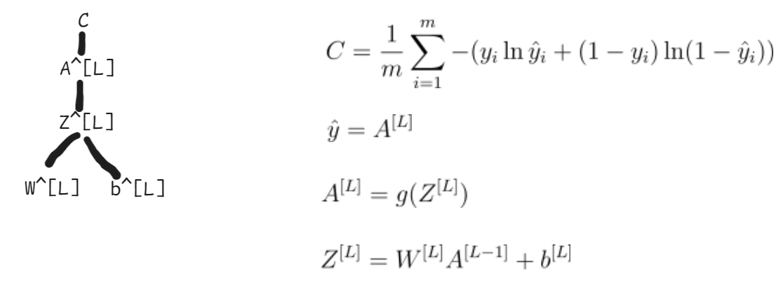
• C depends on the output layer values A⁽ᴸ⁾.
• A⁽ᴸ⁾ depends on pre-activation outputs Z⁽ᴸ⁾.
• Z⁽ᴸ⁾ is directly calculated from W⁽ᴸ⁾ and b⁽ᴸ⁾.

This should look extremely familiar. These are all the calculations for the last layer, and from that we can create a computation graph from C all the way to the weight layer W^[L].

You might be thinking, *Wait, how did we get *ŷ *from *ŷᵢ? And you would be right in noticing how janky the math is. But when we get to coding, that’s when it all works out.

First think of it this way — m ŷᵢ terms is the same thing as the column vector ŷ, so it works out. There’s no succinct way to describe a vector sum in math, so we just use summation notation.

Anyway, from the computation graph above we can use the chain and tree approach to build out these equations (review the partial derivatives chapter if you don’t understand).

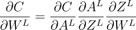
Now I bet you’re *really *glad we’re using matrices instead of doing all these calculations for individual weights and nodes. Imagine all the loops, subscripts, superscripts, etc. if we didn’t use matrices. All we have to do is ensure the matrix dimensions work out well, and we can be 99% sure the math is correct.

Here are the calculations for ∂C/∂A^[L], which may be hard to understand.

**2025 patch: **copy the image below into ChatGPT and ask it to explain the equations to you step by step.

• We don’t keep the summation in the derivative. This is because we are vectorizing, not accessing individual training samples.

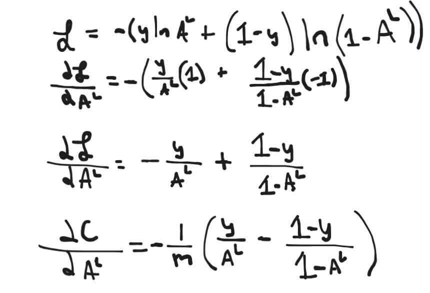
Mom, come pick me up, I’m scared. I know this looks unwieldy, but take it one step at a time.

• Forget about the summation, let’s deal with the individual loss function. All the A^L terms are wrapped in a natural log, so use the chain rule and derivative of ln rules to figure those out.
• We are taking the derivative with respect to A^[L], so we treat that as a variable and everything else as a constant.
• Keep the 1/m term in the cost.

Once we calculate ∂A^[L]/∂Z^[L], you’ll see how we can simplify this monstrous term into something nice and neat.

But first I want to tell you the secret behind checking if your backprop math works. We already know which matrix dimensions we want.

If we are trying to find the gradient of cost with respect to weights in a layer, then that matrix better have the same dimensions as the normal weights matrix.

This is because we update the parameters by subtracting the gradients from them, which is an element-wise operation, requiring both matrices to be the exact same size.

In other words, ∂C/∂W^[L] **must **have the same dimensions as W^[L].

• ∂C/∂A^[L] must have the same dimensions as A^[L].
• ∂C/∂b^[L] must have the same dimensions as b^[L].

This pattern obviously continues for all the layers, but something like ∂Z^[L]/∂W^[L] doesn’t have that restriction because it computes something different entirely. Why don’t you try that calculation out yourself?

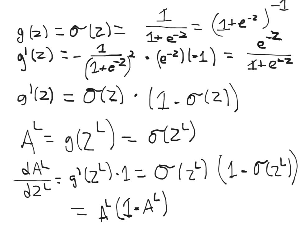
The derivative of sigmoid scares me and I honestly had to look it up, but it evaluates to something nice.

• Use the power rule we learned earlier
• Use chain rule with e^{-z} to get the inner derivative as e^{-z} * -1.
• Use algebra powers to magically realize you can rearrange the monstrous product into just referring back to sigmoid
• Do the same thing for ∂A^[L]/∂Z^[L], where we substitute σ(Z^[L]) for A^[L], since A⁽ᴸ⁾ = g(Z⁽ᴸ⁾) = σ (Z⁽ᴸ⁾).

Now comes the cool part: ∂C/∂A^[L] has the same dimensions as A^[L], and ∂A^[L]/∂Z^[L] has the same dimensions as A^[L] because it’s just element-wise multiplication.

We can multiply these two together element-wise and simplify our calculations to this:

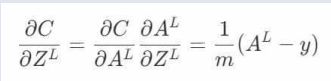
Play around with the algebra and see if you can get the same answer.

We can continue with the chain rule to get our desired calculations at last:

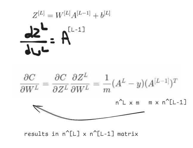
• Find ∂Z^[L]/∂W^[L]. We treat W^[L] as a variable and everything else as a constant, which gets us A^[L-1].
• **Note desired matrix dimensions. **We know that ∂C/∂W^[L] must have the same dimensions as W^[L], which has dimensions n^[L] x n^[L-1].
• Multiply ∂C/∂Z^[L] together with ∂Z^[L]/∂W^[L] as a part of the chain rule to get the answer. To make sure the matrix dimensions match, we transpose the ∂Z^[L]/∂W^[L] calculation.

∂C/∂Z^[L] has the same dimensions as Z^[L], which is n^[L] x m, and A^[L-1] has dimensions n^[L-1] x m.

We know that ∂C/∂W^[L] must have the same dimensions as W^[L], which is an n^[L] x n^[L-1] matrix, so whatever random math we do, we need to end up with those dimensions.

We multiply ∂C/∂Z^[L] by the transpose of A^[L-1] to get a n^[L] x m times m x n^[L-1] matrix multiplication series, giving us the exact dimensions of a n^[L] x n^[L-1] matrix.

Congratulations, you just did your first backprop calculation!

∂C/∂W^[L] represents how we should change the weights in layer L to change the cost most effectively, and with that alone we could reduce the cost. But we have more layers to do, and don’t forget the bias.

The bias is a bit weird though: since we used **broadcasting **before to artificially vectorize the bias matrix for all training samples, during the gradient calculation for biases of a layer we do the opposite — we compress.

Remember that we set b⁽ᴸ⁾ to have dimensions n⁽ᴸ⁾ × m via broadcasting as to do feed-forward for all m training samples at once. In reality, a layer l only has n⁽ˡ⁾ biases, and therefore the gradient of biases for layer L with respect to cost should have dimensions n⁽ᴸ⁾ × 1.

The mathematical representation can’t be vectorized, but just understand we can do it in code.

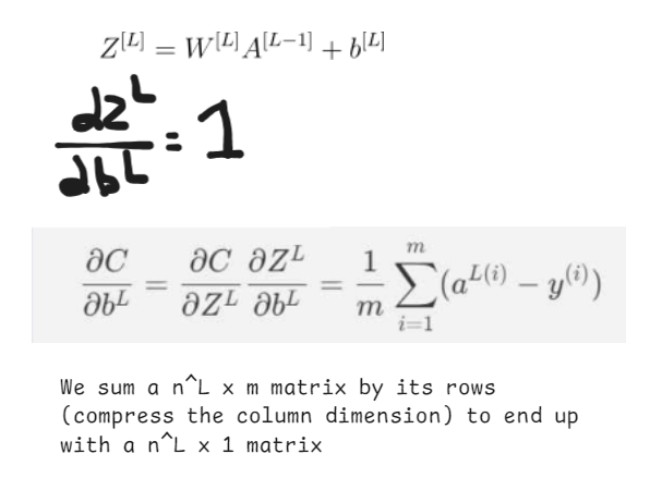
We know that ∂C/∂b^[L] must have the same dimensions as b^[L], which will always be n^[L] x 1, so how do we get there?

• Calculate ∂Z^[L]/∂b^[L], which is just 1, so multiplication with it doesn’t even matter.
• Sum up the ∂C/∂Z^[L] matrix by its rows to end up with a n^[L] x 1 matrix, which I’ll show you how to do in code.

Why does the summation disappear when we’re calculating ∂C/∂W^[L] but magically reappears for calculating ∂C/∂b^[L]? Beats me. ’Tis the cost of vectorization.

What we do know is we ended up with correct matrix dimensions, so you can be at least 99% sure the math is right.

Now you see why knowing the matrix dimensions is so paramount to doing backprop correctly. It really is a lifesaver.

Ok, great. Now what? We only did 1 layer, which is 1/3 of the network. How do we find the gradient of cost with respect to the parameters in the second and even first layers? Just keep calm and chain rule.

Putting the propagation in backpropagation

Going back to feed forward, remember how we could only calculate the final output of the model A^[L] by calculating all the outputs a^[l] for each layer l? That’s our entire computation graph which we can then make partial derivatives from.

We have three layers in our network, so here are the different partial derivatives we would need to calculate:

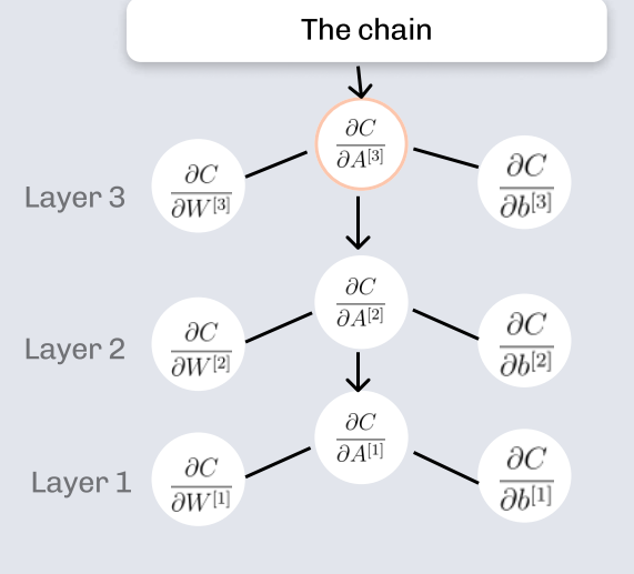
A familiar pattern might be surfacing in your mind right now. Notice how for each layer, we’re calculating almost the same set of partial derivatives?

Let’s follow the computation graph to reach ∂C/∂W^[2]:

I hope this makes sense. Using the feed forward calculations, you can draw computation graph to get a sense of how the equations are connected to each other (W^[L] contributes to Z^[L], Z^[L] contributes to A^[L], etc.) and use the graph/tree to create a chain rule expression.

But this expression looks *real *messy. Why not use a basic aspect of the chain rule to clean it up?

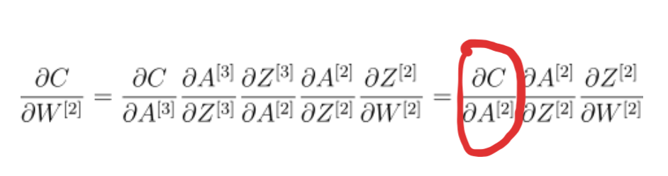
Having just the calculations for layer L=3, we have no idea how to find something like ∂A^[2]/∂Z^[2], but we can definitely find out ∂C/∂A^[2].

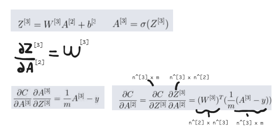
• Look at our feed forward calculation to find out where we use A^[2]. It seems to be in the Z^[3] = W^[3]A^[2] + b^[3] step.
• We already have the value ∂C/∂Z^[3] (which is a n^[3] x m dimensional matrix) since layer 3 is our last layer, so we can multiply that by ∂Z^[3]/∂A^[2] to find ∂C/∂A^[2].
• ∂Z^[3]/∂A^[2] = W^[3], which is the matrix of weights in the third/final layer, which has dimensions n^[3] x n^[2].
• The only way to multiply a n^[3] x m matrix and a n^[3] x n^[2] matrix together is to make the weights matrix the first matrix in the multiplication and then transpose it. So you would get the transpose of W^[3] times whatever ∂C/∂Z^[3] is.

This gives us an n^[2] x m dimensional matrix for ∂C/∂A^[2], which has the same dimensions as A^[2], so we can be sure our math is correct.

The ∂C/∂A^[2] value we calculated is called the **propagator **(I coined this term myself), which we use to continue the backpropagation calculations for each layer. From the propagator we can derive all the important gradient values for a layer we want, like ∂C/∂W^[2] and ∂C/∂b^[2], which we wouldn’t have been able to reach otherwise.

Remember how all our feed forward calculations were essentially the same, but with different dimensions? It’s the exact same thing for backprop, and we can generalize it to any layer l:

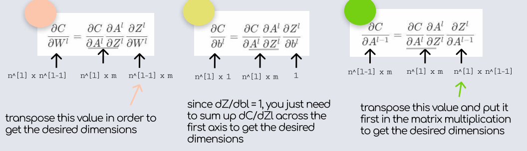
In conclusion, the backprop algorithm is like so:

• Calculate ∂C/∂W^[L] and ∂C/∂b^[L] for the final layer L.
• Calculate the propagator for the penultimate layer L-1 by finding ∂C/∂A^[L-1].
• For all layers l starting from l = L-1, and going until the first layer l=1, calculate ∂C/∂W^[l], ∂C/∂b^[l], and the propagator for the next layer ∂C/∂A^[l-1]

The only caveat for this is that we can substitute A^[0] for X in the code, since they are exactly synonymous (they are both the input layer).

Congrats — we now know exactly what ∇C is: it’s just the gradients of the weights and biases from each layer.

How to update parameters

Now we calculated ∇C, we can finally update our parameters accordingly to reduce the cost.

This leads us to an algorithm called gradient descent, where by going in the opposite direction of the gradient, you can find the minimum of the function.

Remember how the gradient was the slope of a multivariable function, and is the fastest way to increase the function? Then the negative gradient is the exact opposite slope and the fastest way to *decrease *the function, so we always update parameters by the negative of the gradient.

Let’s use the famous “hiking down a cliff” analogy to explain gradient descent.

Pretend that there’s a blind hiker trying to find the quickest way downhill to his valley hometown. At every single second in the journey, he always knows which direction is downhill, but it’s not that simple.

If he takes large steps, the blind hiker might miss a tiny sliver of where the fastest downhill portion is. If he takes extremely small steps, then it’ll take forever for him to descend.

The main idea is that we have **no clue **what the actual cost function looks like, since a cost function for a 10,000 parameter network is 10,000 dimensional. We can only act like the blind hiker, taking small steps and hoping we don’t miss our ticket to the valley.

This is where the idea of the **learning rate **comes in. It regulates how big or small our steps are in a sense.

We multiply the learning rate by the negative of the gradient and then add that to our parameters to update them.

We denote the learning rate as the Greek symbol α (pronounced alpha), which is generally a small value. For the rest of this article, we will use α = 0.01.

Here is how we update the parameters for any layer with gradient descent:

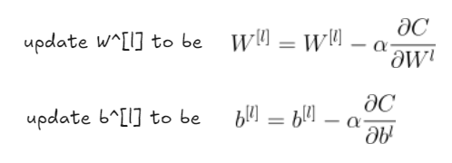
Pretty simple, right?

Because we only take small steps, we have to repeat the backpropagation process over and over again. Don’t worry though — slowly yet surely, we’ll get there.

The training algorithm

This is the last piece of theory we need before we can build the network.

We saw how to calculate an output for the network with feed forward, and even how to update the model parameters with backpropagation.

But those are just the lego pieces — where’s the finished product? It’s nothing but feed forward and backprop a thousand times over.

• Use feed forward to calculate the network output ŷ
• Calculate the cost C from the network output ŷ and the training labels y.
• Save the cost to a list of costs. This is useful in diagnosing if our model is converging to a minimum cost correctly.
• Run backpropagation to compute ∇C (∂C/∂W^[l] and ∂C/∂b^[l] for each layer l).
• Update the parameters using the learning rate you set. A good default is α = 0.01.
• Repeat steps 1–5 100 times, 1000 times, or 10,000,000 times. There is no exact science.

Wait wait, what? Exactly for many iterations are we supposed to run it? This is where computer science becomes more of an art rather than a science. It depends. Here are some ways ML practitioners decide how many iterations to run gradient descent for:

• Choose an arbitrary number like 1000. You can always try different values later. This is the one we’ll use because this article is almost two hours long.
• Run forever until your cost barely stops decreasing. If the cost only reduces by a super small number like 0.001 after a single iteration, you have a good sign to stop gradient descent since you’re likely right on top of the minimum and going any further is pointless.

But relax, you’ve already done the hard part. If you’ve understood all the math, then you should be incredibly proud of yourself. Not many people have gotten to the point of understanding the intuition behind neural networks, let alone tackling the math.

11) Build that network

No ceremonies — I’m tired, I’m sure you are too. Let’s get straight into it. No matter what, you’ll be an entirely new person after this.

Remember this network? Let’s build it.

Feed forward code

Let’s reuse the feed forward code from earlier:

import numpy as np

# 1. initialize the weights and biases to correct shapes with random numbers
L = 3
n = [2, 3, 3, 1]
W1 = np.random.randn(n[1], n[0])
W2 = np.random.randn(n[2], n[1])
W3 = np.random.randn(n[3], n[2])
b1 = np.random.randn(n[1], 1)
b2 = np.random.randn(n[2], 1)
b3 = np.random.randn(n[3], 1)

def prepare_data():
  X = np.array([
      [150, 70],
      [254, 73],
      [312, 68],
      [120, 60],
      [154, 61],
      [212, 65],
      [216, 67],
      [145, 67],
      [184, 64],
      [130, 69]
  ])
  y = np.array([0,1,1,0,0,1,1,0,1,0])
  m = 10
  A0 = X.T
  Y = y.reshape(n[L], m)

  """
  Define X as 10 x 2 = m x n[0] matrix

  Define A_0 as X, the input layer

  Reshape target vector y to be output matrix Y with dims 10 x 1 = m x n[3]
  """

  return A0, Y, m

def cost(y_hat, y):
  """
  y_hat should be a n^L x m matrix
  y should be a n^L x m matrix
  """
  # 1. losses is a n^L x m
  losses = - ( (y * np.log(y_hat)) + (1 - y)*np.log(1 - y_hat) )

  m = y_hat.reshape(-1).shape[0]

  # 2. summing across axis = 1 means we sum across rows, 
  #   making this a n^L x 1 matrix
  summed_losses = (1 / m) * np.sum(losses, axis=1)

  # 3. unnecessary, but useful if working with more than one node
  #   in output layer
  return np.sum(summed_losses)

def g(z):
  return 1 / (1 + np.exp(-1 * z))

def feed_forward(A0):
  # layer 1 calculations
  Z1 = W1 @ A0 + b1
  A1 = g(Z1)

  # layer 2 calculations
  Z2 = W2 @ A1 + b2
  A2 = g(Z2)

  # layer 3 calculations
  Z3 = W3 @ A2 + b3
  A3 = g(Z3)

  cache = {
      "A0": A0,
      "A1": A1,
      "A2": A2
  }

  return A3, cache

If you notice, I made some modifications to our feed forward function — instead of just returning the prediction ŷ, I decided to also return the values A0, A1, and A2.

This is because we need those values for the backpropagation calculations, and returning them along with the feed forward is much easier.

When setting up the data, we get back our X (or A0), y, and the number of training samples m.

A0, Y, m = prepare_data()

Layer L calculations

def backprop_layer_3(y_hat, Y, m, A2, W3):
  A3 = y_hat

  # step 1. calculate dC/dZ3 using shorthand we derived earlier
  #     dC/dZ3 = dC/dA3 * dA3/dZ3
  dC_dZ3 = (1/m) * (A3 - Y)
  assert dC_dZ3.shape == (n[3], m)

  # step 2. calculate dC/dW3 = dC/dZ3 * dZ3/dW3 
  #   we matrix multiply dC/dZ3 with (dZ3/dW3)^T
  dZ3_dW3 = A2
  assert dZ3_dW3.shape == (n[2], m)

  dC_dW3 = dC_dZ3 @ dZ3_dW3.T
  assert dC_dW3.shape == (n[3], n[2])

  # step 3. calculate dC/db3 = np.sum(dC/dZ3, axis=1, keepdims=True)
  dC_db3 = np.sum(dC_dZ3, axis=1, keepdims=True)
  assert dC_db3.shape == (n[3], 1)

  # step 4. calculate propagator dC/dA2 = dC/dZ3 * dZ3/dA2
  dZ3_dA2 = W3 
  dC_dA2 = W3.T @ dC_dZ3
  assert dC_dA2.shape == (n[2], m)

  return dC_dW3, dC_db3, dC_dA2

All we’re doing here is translating the math into code, one to one.

The backpropagation calculations for the final layer take in the following parameters:

• y_hat : the model’s prediction. We rename this to A3 so we can write code just like how we did our math. This has dimensions n^[L] x m.
• Y : the target label. This has dimensions n^[L] x m.
• m : the number of training samples. Not necessary to pass it in, but I wanted to be explicit.
• A2 : The A^[2] activation layer matrix is needed for the ∂Z^[3]/∂W^[3] calculation.
• W3 : We could have just referenced this value globally, but I decided to pass it in to be explicit. Needed for the propagator value.

The backprop calculations for layer L return these values:

• dC_dW3: the partial derivative of the cost with respect to the weights in layer 3. We use this value to adjust the weights in layer 3.
• dC_db3: the partial derivative of the cost with respect to the biases in layer 3. We use this value to adjust the biases in layer 3.
• dC_dA2: the propagator term that lets us continue the chain so we can calculate the derivatives in layer 2.

Just some basic reminders:

• The assert statement is just checking if the matrix dimensions are right. If they are not right, the code will throw an error to let us know.
• The @ symbol means matrix multiplication
• When we use np.sum(some_arr, axis=1), it means we are crunching down on the rows to compress it into an n^[l] x 1 column vector for some layer l.

Here’s a little taste of what the code looks like:

y_hat, cache = feed_forward(A0)
dC_dW3, dC_db3, dC_dA2 = backprop_layer_3(
  y_hat, 
  Y, 
  m, 
  A2= cache["A2"], 
  W3= W3
)

Rest of the layers

def backprop_layer_2(propagator_dC_dA2, A1, A2, W2):

  # step 1. calculate dC/dZ2 = dC/dA2 * dA2/dZ2

  # use sigmoid derivation to arrive at this answer:
  #   sigmoid'(z) = sigmoid(z) * (1 - sigmoid(z))
  #     and if a = sigmoid(z), then sigmoid'(z) = a * (1 - a)
  dA2_dZ2 = A2 * (1 - A2)
  dC_dZ2 = propagator_dC_dA2 * dA2_dZ2
  assert dC_dZ2.shape == (n[2], m)

  # step 2. calculate dC/dW2 = dC/dZ2 * dZ2/dW2 
  dZ2_dW2 = A1
  assert dZ2_dW2.shape == (n[1], m)

  dC_dW2 = dC_dZ2 @ dZ2_dW2.T
  assert dC_dW2.shape == (n[2], n[1])

  # step 3. calculate dC/db2 = np.sum(dC/dZ2, axis=1, keepdims=True)
  dC_db2 = np.sum(dC_dZ2, axis=1, keepdims=True)
  assert dC_db2.shape == (n[2], 1)

  # step 4. calculate propagator dC/dA1 = dC/dZ2 * dZ2/dA1
  dZ2_dA1 = W2
  dC_dA1 = dZ2_dA1.T @ dC_dZ2
  assert dC_dA1.shape == (n[2], m)

  return dC_dW2, dC_db2, dC_dA1

def backprop_layer_1(propagator_dC_dA1, A1, A0, W1):

  # step 1. calculate dC/dZ1 = dC/dA1 * dA1/dZ1

  # use sigmoid derivation to arrive at this answer:
  #   sigmoid'(z) = sigmoid(z) * (1 - sigmoid(z))
  #     and if a = sigmoid(z), then sigmoid'(z) = a * (1 - a)
  dA1_dZ1 = A1 * (1 - A1)
  dC_dZ1 = propagator_dC_dA1 * dA1_dZ1
  assert dC_dZ1.shape == (n[1], m)

  # step 2. calculate dC/dW1 = dC/dZ1 * dZ1/dW1 
  dZ1_dW1 = A0
  assert dZ1_dW1.shape == (n[0], m)

  dC_dW1 = dC_dZ1 @ dZ1_dW1.T
  assert dC_dW1.shape == (n[1], n[0])

  # step 3. calculate dC/db1 = np.sum(dC/dZ1, axis=1, keepdims=True)
  dC_db1 = np.sum(dC_dW1, axis=1, keepdims=True)
  assert dC_db1.shape == (n[1], 1)

  return dC_dW1, dC_db1

You should hopefully see by now how we’re doing the same thing over and over again. At its core, backprop is repetitive. Although we’re being rigid with three layers, it’s trivial to expand that to an arbitrary amount of layers if you know the math.

The backprop calculation for layer 2 takes in the propagator we calculated in layer L and produces the derivatives for layer 2 and the propagator for the next layer.

We then end the backprop process in layer 1.

Here’s how the chain of calling the backprop functions would look like in code:

y_hat, cache = feed_forward(A0)

dC_dW3, dC_db3, dC_dA2 = backprop_layer_3(
    y_hat, 
    Y, 
    m, 
    A2= cache["A2"], 
    W3= W3
)

dC_dW2, dC_db2, dC_dA1 = backprop_layer_2(
    propagator_dC_dA2=dC_dA2, 
    A1=cache["A1"],
    A2=cache["A2"],
    W2=W2
)

dC_dW1, dC_db1 = backprop_layer_1(
    propagator_dC_dA1=dC_dA1, 
    A1=cache["A1"],
    A0=cache["A0"],
    W1=W1
)

Now let’s build our network:

The training begins

def train():
  # must use global keyword in order to modify global variables
  global W3, W2, W1, b3, b2, b1

  epochs = 1000 # training for 1000 iterations
  alpha = 0.1 # set learning rate to 0.1
  costs = [] # list to store costs

  for e in range(epochs):
    # 1. FEED FORWARD (calculates all A1, A2, A3)
    y_hat, cache = feed_forward(A0)

    # 2. COST CALCULATION
    error = cost(y_hat, Y)
    costs.append(error)

    # 3. BACKPROP CALCULATIONS

    dC_dW3, dC_db3, dC_dA2 = backprop_layer_3(
        y_hat, 
        Y, 
        m, 
        A2= cache["A2"], 
        W3=W3
    )

    dC_dW2, dC_db2, dC_dA1 = backprop_layer_2(
        propagator_dC_dA2=dC_dA2, 
        A1=cache["A1"],
        A2=cache["A2"],
        W2=W2
    )

    dC_dW1, dC_db1 = backprop_layer_1(
        propagator_dC_dA1=dC_dA1, 
        A1=cache["A1"],
        A0=cache["A0"],
        W1=W1
    )

    # 4. UPDATE WEIGHTS
    W3 = W3 - (alpha * dC_dW3)
    W2 = W2 - (alpha * dC_dW2)
    W1 = W1 - (alpha * dC_dW1)

    b3 = b3 - (alpha * dC_db3)
    b2 = b2 - (alpha * dC_db2)
    b1 = b1 - (alpha * dC_db1)

    if e % 20 == 0:
      print(f"epoch {e}: cost = {error:4f}")

  return costs

This allows us to get the cost of the neural network on each iteration.

costs = train()

How do we know if our neural network worked? Well if the cost decreased, that’s a pretty good indicator we improved on our training data. Let’s check it out:

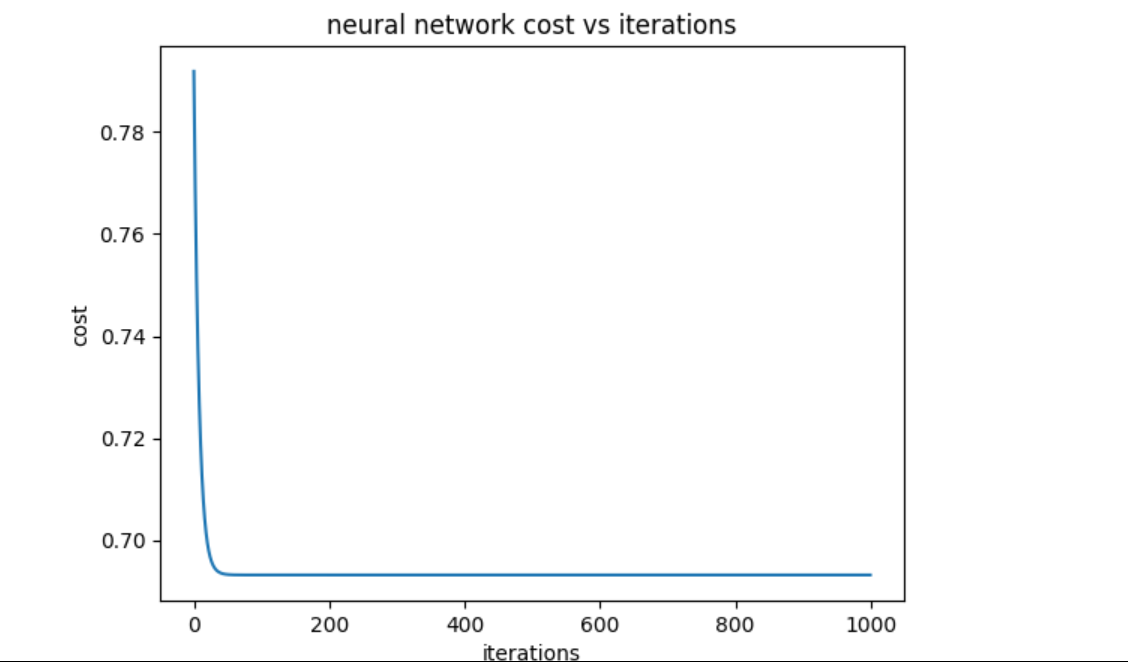
We flatlined after about 30 epochs, so it seems the 1000 iterations was unnecessary.

A Challenge: Challenge 1

Now you know how to build a neural network from scratch. You didn’t just watch me do it (right?) — you tackled the math, battled it and won.

In a world where data scientists are being paid 200k a year just to use scikit-learn without any thought behind it, you forced yourself to go deeper. Not anybody can do that, so revel in the glory.

But are you willing to go deeper?

Here’s a challenge — use the exact same training data to build a neural network, but follow these specifications:

• Generalize the network to work with any amount of layers. Create a function that takes in any number of layers, each with any number of nodes. Return the appropriately sized weights, biases, and other architectural notation as a result.

If you can create a neural network that isn’t hardcoded with a specified number of layers and nodes, then you can call yourself an ML engineer — trust me, the amount you’ve learned is already astounding and far more impressive than whatever Scikit-Learn $200k salary code monkey is doing in Silicon Valley.

The only concepts in artificial intelligence more complicated than building a neural network from scratch is, well … more complicated neural networks — and maybe SVMs (Support Vector Machines).

A Challenge: Challenge 2

You might notice that your network isn’t performing so well, and it might take a long time for the cost to flatline. Why is that?

Well there’s one machine learning concept that’s somewhat inessential for neural network training, but it sure helps.

**Standard scaling **is a way of scaling feature data on different scales so that all features have similar numerical ranges. Without standard scaling, wildly different numerical ranges can slow down learning because the gradient will either explode (get way too big) or vanish (get way too small). After all, the gradient depends on the node/neuron values, so the scale of those will mean the gradient would have a similar scale.

For example, let’s go back to our training data example:

X = np.array([
      [150, 70],
      [254, 73],
      [312, 68],
      [120, 60],
      [154, 61],
      [212, 65],
      [216, 67],
      [145, 67],
      [184, 64],
      [130, 69]
  ])

Notice how the weight (first column) and height (second column) are on completely different scales?

• The weight feature ranges broadly from 130 all the way to 254.
• The height feature is on a smaller range, from 61 to 73.

Doing neural network training with features on vastly different scales slows down training to a halt, and although a network will *still *learn without scaling, it might take a hundred years to do so without it. After all, a neural network is all about turning dials. Vastly different numerical scales may make turning those knobs take longer to make a noticeable change, but it’ll still happen.

Standard scaling just follows a basic formula following these steps:

• Find the mean of all the feature values. For height, this is 66.4 inches.
• Find the standard deviation of all the feature values. For height, this is 3.8 inches.
• For each data point in the feature, use this formula: (data point — mean) divided by standard deviation.

The mathematical way looks like so:

• xᵢ: the i’th data point of the feature.
• μ: the mean of the feature.
• σ: the standard deviation of the feature.

If you standard scale all feature values for all features, you’ll notice something interesting — every single feature now has a mean = 0 and standard deviation = 1.

Every feature that is standard scaled will be in the same numerical range, no matter what. Basically each number in a standard scaled feature will be between -5 and 5, with most data points hovering around 0, 1, or -1. This idea relates to a normal distribution from statistics, but that’s not important.

Once the data is nicely standard scaled, training will go much faster. Your challenge is to implement this in Python. Hint: use Numpy or use ChatGPT.

Bonus: Why do neural networks work?

In this article I showed you how a neural network tries to solve problems by descending the gradient, turning the knobs and dials it has at its disposal. But why neural networks specifically?

There are hundreds of machine learning algorithms, some following this idea of knobs, dials, and gradient descent, while others do something entirely different.

Neural networks are great function approximators, which is important because you can describe ANY problem in humanity like a function.

Want to know if you have lung cancer? Well, that’s just a function f that takes in 35+ variables such as medical history, previous medications, age, weight, and prior smoking history. Some of these variables will be more influential in the equation, like smoking history as compared to weight. The function f will just spit out 0 or 1 — positive or negative diagnosis for lung cancer.

We could graph this function to get essentially a perfect mapping of a person’s health variables to their likelihood of having cancer, but we are not 70-dimensional beings who can visualize that (I wish).

In fact, we’ll *never *achieve the perfect mapping of a person to their cancer output. Here’s why:

• We don’t know which features actually contribute to cancer and which ones are extraneous. Does weight actually matter? Maybe your innocent deodorant caused your cancer.
• We will never have enough data. It is **impossible **to obtain a perfect mapping function if we don’t have all the data. We never recorded people with lung cancer from 4000 BCE — 1960 CE, so all that training data is lost. All we have is essentially a sample of a population, which will always be a probabilistic estimate instead of a perfect, concrete value.

If you’ve read this entire article, then it’s time to use big boy/girl terms now.

The main idea of machine learning is to approximate the unknown target function using this process: 1) Get lots of high quality data. 2) Choose a machine learning model. 3) Train the model.

Neural networks are designed to have hundreds or thousands of variables in the form of their weights. While this initially seems like a random choice, the secret of a neural network’s power lies in its flexibility.

Through gradient descent, it can find out which knobs and dials are actually important and focus on tuning those and which ones are unimportant and thus set those values to 0.

This is why neural networks are the famous machine learning model everybody’s heard of. You don’t have to have any assumptions about what the mathematical function representation of a problem might look like. You can choose a 1000 dimensional function (has 1000 features) and through adequate training, the network will morph its function representation to only care about 5 dimensions and ignore the rest.

Is it linear? Polynomial? Exponential — who cares? The unique design of a neural network allows it to approximate any mathematical function as long as you train it with enough data.

Other less flexible machine learning models like linear regression are worse than neural networks because they can’t adapt to more complex problems that require polynomial or exponential representations — they can only ever draw a straight line.

Here’s an animated example of what I mean:

[Embedded content](The ReLu activation function — another choice instead of sigmoid — allows the neural network to approximate any function in existence)

Bonus: demystifying ChatGPT

What about ChatGPT — how does that work?

Well going back to our principle of neural networks being universal function approximators, we can say LLMs (large language models) like ChatGPT are expert approximators of the human language.

What? How do we approximate the human language? And much less represent it as a math function?

Well it’s not like the words us humans say to each other are random: it’s expected that a “hello” garners a “hi” back. If you say “how do you do,” to someone, “jkahjasdjfkafauasdfj” isn’t a valid response back, and maybe even garners a “huh?”

Language follows patterns and thus can be mapped to a mathematical function.

Somewhere out there in the universe is a f(X) that takes millions of features representing all the factors that influence human language and adequate responses to human text.

Yes, that golden ideal function probably has millions of different unknown features, but that’s why ChatGPT works so well: you don’t have to know those features.

Does cancer really just depend on your height and weight? If so, send Shaquille O’Neil to the hospital.

Similarly, language could depend on a person’s mood, a bee buzzing next to them, previous conversational context, tone, grammar, or even the weather.

What do you get when you slam millions of dollars and petabytes of training data into a model that trains continuously for months on end? Given a hell of a long time to do gradient descent, you’ll arrive at an excellent approximation of the human language.

ChatGPT is not a simple neural network with input layers and hidden layers. Trust me — it’s much more complicated.

But regardless of the insanity behind such architectures, they all boil down to mathematical functions, approximations of the ideal functions we want to target.

Think of anything in your life that follows patterns. Now maybe you can automate it with your own neural network.

So long, partner

I hope you’ve learned something today and made yourself proud. When I was able to build a neural network on my own, it changed the way I viewed myself. For years I’ve struggled, telling myself I wasn’t smart enough, but if you work hard, you really can do it.

If I was of any help at all, I would appreciate if you could share this article — I spent way too much time writing it.

If you want to see all the math in slides you can refer to again and again, here you go:

**Neural Networks Mathematics: From Feed Forward To Backpropagatio**n Neural Networks Mathematics: From Feed Forward To Backpropagation - Download as a PDF or view online for freewww.slideshare.net

Shameless self promotion

This is free:

**Master JavaScript 2024: 2 Coding Notebook**s *Master JavaScript ES6 through this comprehensive Google Colab notebook bundle🚀 Welcome to the first of its kind online…*musicandcoding.gumroad.com

*Not *free lol, but less than $5:

**Expert React Developer Bundle 2024: Become a Reactjs expert**! *🚀 Unlock the full potential of React.js with my Ultimate React.js Mastery Bundle! This comprehensive collection of…*musicandcoding.gumroad.com

**Learn TypeScript Fundamentals: Comprehensive Coding Noteboo**k *Master TypeScript Fundamentals through this comprehensive Google Colab notebook🚀 Welcome to the first-ever online…*musicandcoding.gumroad.com

**NodeJS Mastery 2024 - 3 Digital Coding Notebook**s *Product Title: Ultimate Node.js Mastery Bundle: Beginner to Advanced🚀 Elevate your Node.js skills with my Ultimate…*musicandcoding.gumroad.com

**Learn Python in 2024: Online Coding Noteboo**k *Learn python with this amazing google colab online notebook! Use my 5 years of Python experience - all compiled into…*musicandcoding.gumroad.com

A message from our Founder

**Hey, Sunil here. I wanted to take a moment to thank you for reading until the end and for being a part of this community.

Did you know that our team run these publications as a volunteer effort to over 3.5m monthly readers? We don’t receive any funding, we do this to support the community. ❤️

If you want to show some love, please take a moment to **follow me on LinkedIn, TikTok, **Instagra**m. You can also subscribe to our **weekly newslette**r.

And before you go, don’t forget to clap and follow the writer️!

Comments

Loading comments…