The Difference Between Back Propagation and Forward Propagation in Deep Learning

Deep Learning, a subset of machine learning, has revolutionized how we approach complex problems in various fields, from image recognition to natural language processing. Central to the operation of deep learning algorithms are two fundamental concepts: forward propagation and back propagation. In this article, we will delve into these concepts, unraveling their intricacies and differences.

Understanding Deep Learning

Deep learning involves the use of neural networks, which are computing systems vaguely inspired by the human brain’s structure. These networks are composed of layers of interconnected nodes, or neurons, that process and transmit data. Understanding how data flows and is processed within these networks is crucial for grasping the concepts of forward and back propagation.

Forward Propagation

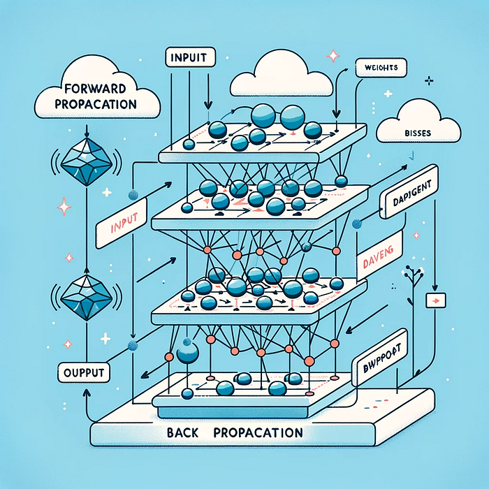
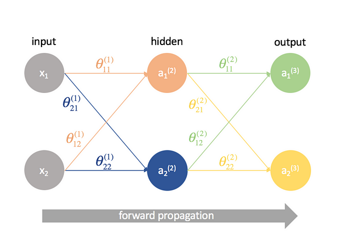
Forward propagation is the initial phase of data processing in a neural network. Here, input data is fed into the network and passed through various layers. Each neuron in these layers processes the input and passes it to the next layer, ultimately leading to the output layer. This process is linear and straightforward, moving in one direction: from input to output.

Back Propagation

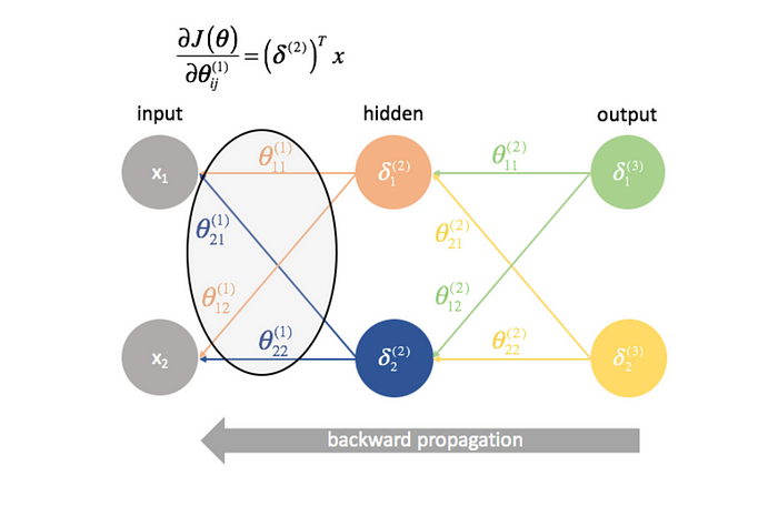
Back propagation, on the other hand, is the learning phase. Once the forward propagation is complete and an output is produced, the network compares this output to the desired outcome. The difference, or error, is then used to adjust the network’s weights and biases. This process is iterative and involves moving backward through the network, fine-tuning it to minimize the error.

Comparing Forward and Back Propagation

While forward propagation is about data processing and producing an output, back propagation is about learning from errors and improving the network’s accuracy. Both are integral to the functioning of a neural network, each serving a distinct yet interconnected role.

Challenges and Limitations

Despite their effectiveness, both methods come with challenges. Forward propagation can become computationally intensive with complex networks, while back propagation can suffer from issues like vanishing gradients, where the gradients used in the learning process become too small to make significant changes in the network.

Implementation example

This example will create a basic neural network to classify handwritten digits from the MNIST dataset, a common benchmark in deep learning.

The MNIST dataset contains 28x28 pixel grayscale images of handwritten digits (0 through 9). We’ll use a simple neural network with one hidden layer for this demonstration. TensorFlow will handle both the forward and back propagation steps as part of the training process.

First, ensure you have TensorFlow installed. You can install it via pip:

pip install tensorflow

Now, let’s proceed with the example:

import tensorflow as tffrom tensorflow.keras.datasets import mnistfrom tensorflow.keras.models import Sequentialfrom tensorflow.keras.layers import Dense, Flattenfrom tensorflow.keras.optimizers import SGD# Load the MNIST dataset  
(x_train, y_train), (x_test, y_test) = mnist.load_data()  
  
# Normalize the datax_train, x_test = x_train / 255.0, x_test / 255.0  
  
# Build a Sequential model  
model = Sequential([  
    Flatten(input_shape=(28, 28)), # Flatten the 28x28 images Dense(128, activation='relu'), # Hidden layer with 128 neurons and ReLU activation Dense(10, activation='softmax') # Output layer with 10 neurons (one for each class) and softmax activation  
])  
  
# Compile the model  
model.compile(optimizer=SGD(),   
              loss='sparse_categorical_crossentropy',   
              metrics=['accuracy'])  
  
# Train the model  
model.fit(x_train, y_train, epochs=5)  
  
# Evaluate the model  
loss, accuracy = model.evaluate(x_test, y_test)  
print(f"Test Accuracy: {accuracy * 100:.2f}%")

In this script:

Data Preparation: The MNIST dataset is loaded and normalized.
Model Building: A Sequential model is created with one hidden layer.
Forward Propagation: Occurs during the model’s training (model.fit) and prediction phases. Data flows from the input layer through the hidden layers to the output layer.
Back Propagation: Happens automatically during training. TensorFlow adjusts the weights and biases based on the loss function (sparse_categorical_crossentropy in this case) using the Stochastic Gradient Descent (SGD) optimizer.