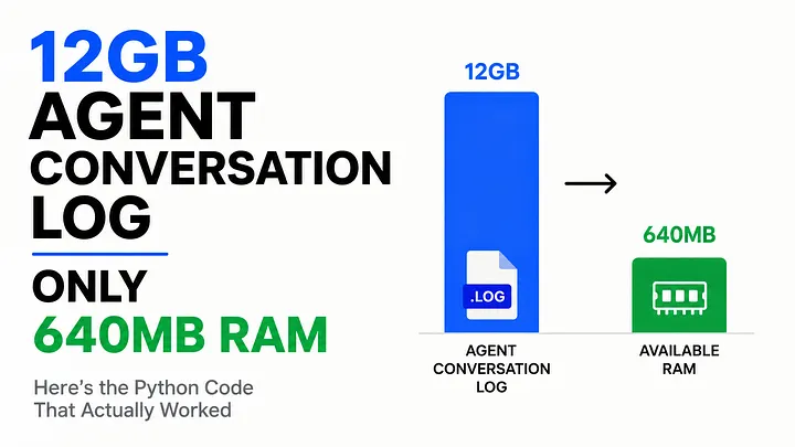
12GB of nested AI agent logs. 640MB of RAM. Here is the streaming pipeline that actually survived.
How do you process a 12GB JSONL file on a server with just 640MB of RAM?
Most developers reach for pd.read_json() or json.load(). That works until your file is larger than memory. Then the process slows to a crawl, crashes, or gets killed before parsing finishes.
This is a problem many AI teams discover the hard way. Agent logs grow fast. Every conversation, tool call, reasoning step, and observation gets stored. After a few months in production, those logs can become massive.
I ran into this while building a retrieval dataset for a RAG pipeline. The source file was a 12GB nested JSONL export. Available RAM was only 640MB.
The obvious solution failed immediately. The approach that worked handled the file efficiently, cleaned and transformed records on the fly, and never came close to exhausting memory.
Here is the exact method, why the common approach breaks, and which strategy to use for different workloads.
Why Normal Loading Fails
Agent conversation logs are not simple tables. Each line in a JSONL file can contain an entire interaction: user messages, reasoning traces, tool calls, tool outputs, token usage, latency metrics, and other nested metadata.
That complexity is exactly why the obvious solution fails.
When you run pd.read_json(), Pandas attempts to parse and organize the entire dataset at once. Every nested structure must be loaded into memory before a usable DataFrame can even exist.
json.load() is even more dangerous. It builds a complete Python object tree for the entire file before you can process a single record. Every dictionary, list, string, and nested object adds overhead, causing memory usage to balloon far beyond the file's size on disk.
The result surprises most developers. A 12GB JSONL file can easily consume 25 to 40GB of RAM during parsing.
On a machine with only 640MB available, there is no gradual slowdown. The process simply runs out of memory and dies before any useful work gets done.
The Core Idea: Stream, Don’t Load
The solution is not a better parser. It is a different way of thinking about the problem.
If the file is larger than available memory, stop trying to load the whole thing.
Instead, stream it.
Read one record. Process it. Write the result. Discard it. Repeat millions of times if necessary.
Memory usage stays almost constant because only a tiny working set exists at any given moment. It does not matter whether the file is 12GB, 120GB, or larger. The process scales because the dataset never lives in memory all at once.
This approach is especially effective for agent conversation logs because JSONL was designed for streaming. Every conversation turn is stored as a separate line, making it possible to parse records independently without touching the rest of the file.
Once you adopt that mindset, handling massive log files becomes surprisingly straightforward.
There are three practical approaches I use, ranging from simple line-by-line processing to fully optimized data pipelines. Which one you choose depends on the size of the data, the complexity of the transformations, and how often the workflow needs to run.
Method 1: Pandas with chunksize (Quick Fix)
Pandas can stream JSONL files using lines=True and chunksize, turning the read operation into an iterator that yields small DataFrames instead of one massive one.
Rather than loading the entire dataset into memory, Pandas processes it in manageable batches. You can clean, filter, and transform each chunk before moving to the next, keeping memory usage tied to the chunk size instead of the file size.
import pandas as pd

chunk_size = 5000
output_path = "cleaned_agent_logs.parquet"

for chunk in pd.read_json(
    "agent_logs_12gb.jsonl",
    lines=True,
    chunksize=chunk_size
):
    # Filter out incomplete or failed agent runs
    chunk = chunk[chunk["status"] == "completed"]

    # Flatten tool call counts for quick analysis
    chunk["tool_call_count"] = chunk["tool_calls"].apply(
        lambda calls: len(calls) if isinstance(calls, list) else 0
    )

    chunk.to_parquet(output_path, engine="pyarrow", index=False)
This works well for moderately large files and is often enough to stop the immediate crash. The downside is that Pandas still builds a full DataFrame for every chunk, parsing all nested fields into Python objects first.
With agent logs containing deeply nested tool calls and reasoning traces, memory usage can still spike higher than expected if the chunk size is not tuned carefully. It is a useful quick fix, but not usually the approach you want powering a production pipeline at this scale.
Method 2: ijson for True Streaming
ijson parses JSON incrementally, emitting events as it encounters them rather than building the full structure first. For agent logs where you only need specific fields out of a deeply nested structure, this avoids loading the parts you do not need at all.
import json

def stream_agent_logs(filepath):
    with open(filepath, "rb") as f:
        for line in f:
            try:
                yield json.loads(line)
            except json.JSONDecodeError:
                continue

def extract_for_rag(record):
    if record.get("status") != "completed":
        return None
    return {
        "conversation_id": record.get("id"),
        "user_message": record.get("input", {}).get("message"),
        "final_response": record.get("output", {}).get("text"),
        "tool_calls_made": len(record.get("tool_calls", [])),
    }

output_path = "rag_ready_logs.jsonl"

with open(output_path, "w") as out_file:
    for record in stream_agent_logs("agent_logs_12gb.jsonl"):
        extracted = extract_for_rag(record)
        if extracted:
            out_file.write(json.dumps(extracted) + "\n")
Since the file is line-delimited JSONL, reading line by line with json.loads() per line already gives you most of ijson’s benefit without the added dependency, which is what the example above does. True ijson becomes more valuable when you are dealing with a single massive JSON array rather than line-delimited records, since it lets you stream into the array without ever holding the full list in memory.
Method 3: Polars Lazy Streaming (My Favorite in 2026)
Polars has become the tool I reach for first on anything involving large structured data, and its lazy streaming API is built specifically for this kind of constraint.
import polars as pl

lazy_df = pl.scan_ndjson("agent_logs_12gb.jsonl")

result = (
    lazy_df
    .filter(pl.col("status") == "completed")
    .with_columns([
        pl.col("tool_calls").list.len().alias("tool_call_count"),
        pl.col("output").struct.field("text").alias("final_response"),
    ])
    .select(["id", "final_response", "tool_call_count", "timestamp"])
)

result.sink_parquet("agent_logs_processed.parquet", compression="zstd")
This is where Polars starts to separate itself from the other approaches.
scan_ndjson() creates a lazy query plan instead of reading data immediately. Combined with sink_parquet(), Polars streams transformed results directly to disk, so the full dataset never needs to exist in memory.
The real advantage for agent logs is native support for nested structs and lists. You can extract fields from tool calls, reasoning traces, and metadata directly inside the query plan without writing custom extraction logic. Filtering, transformations, and aggregations are pushed into a single optimized execution pipeline rather than executed as separate memory-intensive steps.
On the 12GB agent log file, this was the only approach that handled the workload comfortably with just 640MB of available RAM, requiring no chunk-size tuning and no manual memory management.
Production-Grade Pipeline I Actually Use
The pipeline I run in production combines a custom generator with batching, giving me control over batch size, error handling, and where partial failures get logged separately rather than crashing the whole run
import json
from itertools import islice

def batch_generator(filepath, batch_size=1000):
    with open(filepath, "r") as f:
        while True:
            batch = list(islice(f, batch_size))
            if not batch:
                break
            yield batch

def process_batch(lines, error_log):
    processed = []
    for line in lines:
        try:
            record = json.loads(line)
            if record.get("status") == "completed":
                processed.append({
                    "id": record["id"],
                    "text": record.get("output", {}).get("text", ""),
                    "tool_calls": len(record.get("tool_calls", [])),
                })
        except (json.JSONDecodeError, KeyError) as e:
            error_log.append(str(e))
    return processed

error_log = []
output_path = "production_ready_logs.jsonl"

with open(output_path, "w") as out_file:
    for batch in batch_generator("agent_logs_12gb.jsonl", batch_size=1000):
        processed = process_batch(batch, error_log)
        for record in processed:
            out_file.write(json.dumps(record) + "\n")

if error_log:
    with open("processing_errors.log", "w") as ef:
        ef.write("\n".join(error_log))
This approach gives up some of the elegance of the Polars solution in exchange for explicit control. Malformed lines get logged instead of crashing the run, batch size is tunable independently of any library’s internal chunking behavior, and the entire pipeline has no dependency beyond the standard library, which matters on constrained production servers where installing additional packages is not always straightforward.
Real Results and Lessons Learned
The naive pd.read_json() approach crashed immediately. Chunked Pandas completed the job, but poorly tuned chunk sizes pushed memory usage to nearly 480MB, leaving very little room for anything else running on the server.
Polars finished the entire pipeline in under 14 minutes while keeping peak memory usage below 200MB. That margin mattered because the same machine was actively running agents and generating new logs during processing.
The custom generator approach took about 22 minutes. It was slower, but it offered the most predictable memory usage and the best resilience when records were malformed.
That last point turned out to be more important than performance. Real agent logs are messy. Crashed agents leave behind truncated JSON lines, interrupted tool call arrays, and schema mismatches between deployments. Those issues appeared far more often than expected.
The biggest lesson was simple: build error handling into the pipeline from day one. With agent logs, malformed data is not an edge case. It is part of the dataset.
Final Verdict
Use chunked Pandas when you need a quick fix and the data is not heavily nested.
Use Polars lazy streaming as the default for agent logs. Its native handling of nested data and low memory usage make it the best choice for most production pipelines.
Use a custom generator and batching approach when you need maximum control over error handling or cannot add external dependencies.
If you are running AI agents in production, this problem is not a matter of if. It is a matter of when. Build the streaming pipeline before the crash forces you to.
Hit a different wall processing agent logs at scale? Drop it in the comments. I read every one. Follow for practical Python solutions to the problems that only appear once AI agents reach production.
Comments
Loading comments…